

Large Scale Learning Challenge
Challenge: 27 February - 27 June 2008
With the exceptional increase in computing power, storage capacity and network bandwidth of the past decades, ever growing datasets are collected in fields such as bioinformatics (Splice Sites, Gene Boundaries, etc), IT-security (Network traffic) or Text-Classification (Spam vs. Non-Spam), to name but a few. While the data size growth leaves computational methods as the only viable way of dealing with data, it poses new challenges to ML methods.
This PASCAL Challenge is concerned with the scalability and efficiency of existing ML approaches with respect to computational, memory or communication resources, e.g. resulting from a high algorithmic complexity, from the size or dimensionality of the data set, and from the trade-off between distributed resolution and communication costs.
Indeed many comparisons are presented in the literature; however, these usually focus on assessing a few algorithms, or considering a few datasets; further, they most usually involve different evaluation criteria, model parameters and stopping conditions. As a result it is difficult to determine how does a method behave and compare with the other ones in terms of test error, training time and memory requirements, which are the practically relevant criteria.
We are therefore organizing a competition, that is designed to be fair and enables a direct comparison of current large scale classifiers aimed at answering the question “Which learning method is the most accurate given limited resources?”. To this end we provide a generic evaluation framework tailored to the specifics of the competing methods. Providing a wide range of datasets, each of which having specific properties we propose to evaluate the methods based on performance figures, displaying training time vs. test error, dataset size vs. test error and dataset size vs. training time.
General
The overall goal is to develop a 2-class classifier such that it achieves a low error in the shortest possible time using as few datapoints as possible.
In order to fairly assess the performances of the SVM-QP solvers, the participants to the SVM tracks are asked to comply with two requirements:
|
Challenge Tasks
The overall goal is to tune your method such that achieves a low test error measured by the area over the precision recall curve in the shortest possible time and using as few datapoints as possible.
Wild Competition TrackIn this track you are free to do anything that leads to more efficient, more accurate methods, e.g. perform feature selection, find effective data representations, use efficient program-code, tune the core algorithm etc. It may be beneficial to use the raw data representation (described below). For each dataset your method competes in you are requested to:
|
SVM TracksTo allow for a comparison w.r.t. to non-SVM solvers, all SVM methods are required to compete in both tracks and therefore for SVMs step 1 is to attack the wild-track task. In addition to what has to be done in the wild track we ask you to do the following experiments.
Here epsilon denotes the relative duality gap (obj_primal-obj_dual)/obj_primal<epsilon=0.01. If your solver has a different stopping condition, choose it reasonably, i.e. such that you expect it to have similar duality gap. While early stopping is OK it may hurt your method in evaluation: If the objective of your svm solver deviates too much from others, i.e. by more than 5% (your_obj-obj_min)/your_obj<0.05, it will get low scores. Note that you have to use the data representation obtained by running the svmlight-conversion script in the second part (model selection) of the experiment. The following values for C/rbf-width shall be used:
Objective values are computed as follows:
Finally, if possible please include all parameters, rbf-tau, epsilon, SVM-C for all experiments in the result file. |
Parallel TrackThe recent paradigm shift of learning from single to multi-core shared memory architectures is the focus of the parallel track. For the parallel track methods have to be trained on 8 CPUs following the rules outlined in the wild track. To assess the parallelization quality, we in addition ask participants to train their method using 1,2,4,8 CPUs on the biggest dataset they can process. Note that the evaluation criteria are specifically tuned to parallel shared memory algorithms, i.e. instead of training time on each CPU you should measure wall-clock-time (including data loading time). In addition data loading time must be specified in a separate field. |
 .
.

Datasets
The raw datasets can be downloaded from ftp://largescale.ml.tu-berlin.de/largescale. The provided script convert.py may be used to obtain a simple (not necessary optimal) feature representation in svm-light format.
Overview of the Raw Datasets |
||||
|---|---|---|---|---|
| Dataset | Training | Validation | Dimensions | Format Description |
| alpha | 500000 | 100000 | 500 |
Files are in ascii format, where each line corresponds to 1 example, i.e. val1 val2 ... valdim\n val1 val2 ... valdim\n ... |
| beta | 500000 | 100000 | 500 | |
| gamma | 500000 | 100000 | 500 | |
| delta | 500000 | 100000 | 500 | |
| epsilon | 500000 | 100000 | 2000 | |
| zeta | 500000 | 100000 | 2000 | |
| fd | 5469800 | 532400 | 900 |
Files are binary, to obtain 1 example read 900 or 1156 bytes respectively (values 0..255) |
| ocr | 3500000 | 670000 | 1156 | |
| dna | 50000000 | 1000000 | 200 |
Files are ascii, each line contains a string of length 200 (symbols ACGT), i.e. CATCATCGGTCAGTCGATCGAGCATC...A\n GTGTCATCGTATCGACTGTCAGCATC...T\n ... |
| webspam | 350000 | 50000 | variable |
Files contains strings (webpages) separated with 0, i.e.
        html foo bar .../html\0
|
Submission Format
We provide an evaluation script that parses outputs and computes performance scores. We use this exact same script to do the live evaluation. It is suggested to run this script locally on a subset of the training data to test whether the submission format is correctly generated and to evaluate the results (note that the script can only be used on data where labels are available, e.g. subsets of the training data). It requires python-numpy and scipy to be installed. Additionally if matplotlib is installed, the performance figures will be drawn.
Additionally the data submission format is described below:
- Wild Competition (download example submission)
dataset_size0 -1 traintime0 testtime0 calibration0 objective C epsilon rfb-tau output0 output1 ... ... dataset_sizeN -1 traintimeN testtimeN calibrationN objective C epsilon rfb-tau output0 output1 ... dataset_sizeN index0 traintime0 testtime0 calibration0 objective C epsilon rfb-tau output0 output1 ... ... dataset_sizeN index9 traintime9 testtime0 calibration9 objective C epsilon rfb-tau output0 output1 ... - SVM Tracks (download example submission)A submission to the SVM track requires to take part in the wild competition, i.e. the submission file must start with the lines required for the wild competition. Then a single empty line announces the SVM-Track specific data:
>a singly empty line here distinguishes wild from model specific track
        dataset_size0 -1 traintime0 testtime0 calibration0 objective C epsilon rfb-tau
        ...
        dataset_sizeN -1 traintimeN testtimeN calibrationN objective C epsilon rfb-tau
        dataset_sizeN index1 traintime1 testtime1 calibration1 objective C epsilon rfb-tau
        ...
        dataset_sizeN index9 traintime9 testtime0 calibration9 objective C epsilon rfb-tau
        dataset_sizeN -2 traintime0 testtime0 calibration0 objective C1 epsilon rfb-tau
        ...
        dataset_sizeN -2 traintimeK testtimeK calibration9 objective CK epsilon rfb-tau

(or -3 and rbf-tau 1 ... K)
- Parallel Track
A submission to the parallel track consists of two parts: The first one has the exact same syntax as the wild track (with time = wall-clock-time). The second part contains the 1,2,4,8 CPU experiment run on the biggest dataset (here C denotes the number of CPUs)
>a singly empty line here distinguishes wild from model specific track
        dataset_sizeN -4 walltimeN dataloadingtimeN calibrationN objective 1 epsilon rfb-tau
        dataset_sizeN -4 walltimeN dataloadingtimeN calibrationN objective 2 epsilon rfb-tau
        dataset_sizeN -4 walltimeN dataloadingtimeN calibrationN objective 4 epsilon rfb-tau
        dataset_sizeN -4 walltimeN dataloadingtimeN calibrationN objective 8 epsilon rfb-tau
Explanation of values (Column by Column)
- Dataset size – Values must match size of dataset or 10^[2,3,4,5,6,7]
- Index values of 0…9 (to distinguish values obtained while optimizing) only for the biggest dataset, -1 otherwise; for the SVM track -2 for the C experiment and -3 for the rbf-tau experiment
- Traintime – Time required for training (without data loading) in seconds / wall-clock time (including data loading) for the parallel track
- Testtime – Time required for applying the classifier to the validation/test data (without data loading) in seconds / data loading time for the parallel track
- Calibration – Score obtained using the provided calibration tool (values should be the same if run on the same machine)
- Method specific value: SVM Objective
- SVM-C / number of CPUs for the parallel track
- SVM-rbf-tau
- SVM epsilon
- use 0 (for SVM Objective, SVM-C, SVM-rbf-tau, SVM epsilon) if not applicable
- for SVM please fill in the different parameters, i.e. SVM objective, SVM-C, rbf-tau and stopping condition epsilon, as the meaning of epsilon may differ please explain in the description what epsilon stands for
- for the linear svm track index -2 should be used when doing the experiment for C
- for the gaussian svm track index -3 should be used when modifying rbf tau
- The following values in columns 10-… must match the size of the validation/test set.
Assessment of the submissions
Different procedures will be considered depending on the track.
Wild Competition
For the Wild track, the ideal goal would be to determine the best algorithm in terms of learning accuracy, depending on the time budget allowed. Accordingly, the score of a participant is computed as the average rank of its contribution wrt the six scalar measures:
 |
This figure measures training time vs. area over the precision recall curve (aoPRC). It is obtained by displaying the different time budgets and their corresponding aoPRC on the biggest dataset. We compute the following scores based on that figure:
|
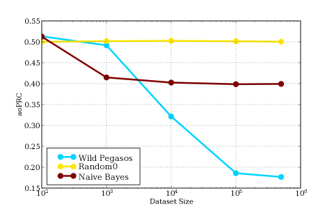 |
This figure measures dataset size vs. area over the precision recall curve (aoPRC). It is obtained by displaying the different dataset sizes and their corresponding aoPRC that the methods achieve. We compute the following scores based on that figure:
|
 |
This figure measures dataset size vs. training time. It is obtained by displaying the different dataset sizes and the corresponding training time that the methods achieve. We compute the following scores based on that figure:
|
SVM Tracks
For the SVM track, the point is to determine the best tradeoff between the computational effort and the learning accuracy. Accordingly, the score of a participant is computed as the average rank of its contribution wrt the five scalar measures
- Minimal objective
- Area under the Time vs. Objective Curve
- Time to reach objective within 5% tolerance, i.e. minimal t for (t,obj) with (obj-overal_min_objective)/obj<0.05
- Average Training Time for all C/Sigma
- Computational Effort (scaling with dataset size)
Validation Results
Overall Ranking
| Rank | Score | Submitter | Title | Date |
|---|---|---|---|---|
| 1 | 4.40 | chap – Olivier Chapelle | Newton SVM | 02.05.2008 20:57 CET |
| 2 | 5.20 | yahoo – Olivier Keerthi | SDM SVM L2 | 19.06.2008 13:49 CET |
| 3 | 5.60 | yahoo – Olivier Keerthi | SDM SVM L1 | 18.06.2008 19:28 CET |
| 4 | 5.80 | antoine – Antoine Bordes | SgdQn | 16.06.2008 14:21 CET |
| 5 | 7.90 | kristian – Kristian Woodsend | IPM SVM 2 | 23.06.2008 15:10 CET |
| 5 | 7.90 | kristian – Kristian Woodsend | Interior Point SVM | 16.06.2008 21:56 CET |
| 7 | 8.60 | beaker – Gavin Cawley | LR | 19.06.2008 13:21 CET |
| 8 | 9.90 | ker2 – Porter Chang | CTJ LSVM01 | 20.06.2008 03:31 CET |
| 9 | 10.70 | rofu – Rofu yu | test | 10.06.2008 16:31 CET |
| 10 | 11.70 | MB – Marc Boulle | Averaging of Selective Naive Bayes Classifiers final | 20.06.2008 12:06 CET |
| 11 | 11.90 | beaker – Gavin Cawley | ORRR | 12.06.2008 16:13 CET |
| 11 | 11.90 | rofu – Rofu yu | liblinear | 25.06.2008 11:57 CET |
| 13 | 12.60 | MB – Marc Boulle | Averaging of Selective Naive Bayes Classifiers | 27.05.2008 14:56 CET |
| 14 | 14.00 | garcke – Jochen Garcke | AV SVM | 02.06.2008 13:41 CET |
| 15 | 14.10 | aiiaSinica – Han-Shen Huang | CTJ LSVM | 19.06.2008 04:16 CET |
| 16 | 14.70 | fravoj – Vojtech Franc | Random | 18.02.2008 15:29 CET |
| 17 | 15.20 | beaker – Gavin Cawley | WRRR | 24.06.2008 13:12 CET |
| 18 | 15.50 | rofu – Rofu yu | L1 | 13.06.2008 13:17 CET |
| 19 | 16.30 | antoine – Antoine Bordes | LaRankConverged | 13.06.2008 19:11 CET |
| 20 | 17.20 | beaker – Gavin Cawley | ORRR Ensemble | 15.06.2008 16:54 CET |
| 21 | 17.40 | ker2 – Porter Chang | CTJ LSVM02 | 25.06.2008 14:38 CET |
| 22 | 18.80 | fravoj – Vojtech Franc | ocas | 25.06.2008 14:28 CET |
| 22 | 18.80 | antoine – Antoine Bordes | Larank | 13.06.2008 14:37 CET |
| 24 | 19.20 | beaker – Gavin Cawley | rr | 06.06.2008 21:14 CET |
| 24 | 19.20 | garcke – Jochen Garcke | AV SVM single | 25.06.2008 15:58 CET |
| 26 | 19.30 | aiiaSinica – Han-Shen Huang | linearSVM01 | 11.06.2008 03:42 CET |
| 26 | 19.30 | xueqinz – Xueqin Zhang | CHSVM | 07.01.2009 01:27 CET |
| 28 | 19.60 | garcke – Jochen Garcke | AV SVM 500k | 10.06.2008 11:49 CET |
| 28 | 19.60 | garcke – Jochen Garcke | AV SVM rbf track | 23.06.2008 14:23 CET |
| 30 | 19.70 | fravoj – Vojtech Franc | Stochastic SVM | 18.02.2008 14:29 CET |
| 31 | 20.30 | aiiaSinica – Han-Shen Huang | linearSVM03 | 16.06.2008 05:58 CET |
| 32 | 20.40 | rofu – Rofu yu | Coordinate descent dual l1 linear svm | 10.06.2008 15:21 CET |
| 33 | 20.50 | aiiaSinica – Han-Shen Huang | sLsvm | 17.06.2008 08:51 CET |
| 34 | 20.70 | ker2 – Porter Chang | CTJsvm | 21.01.2009 12:42 CET |
| 35 | 20.80 | aiiaSinica – Han-Shen Huang | lsvm04 | 16.06.2008 06:57 CET |
| 36 | 21.00 | ker2 – Porter Chang | anSGD | 05.01.2009 08:21 CET |
| 37 | 21.10 | xueqinz – Xueqin Zhang | CHSVM4 | 14.01.2009 06:13 CET |
| 38 | 21.30 | fravoj – Vojtech Franc | random2 | 25.06.2008 14:48 CET |
| 39 | 21.40 | bernhardP – Bernhard Pfahringer | Random model trees | 11.06.2008 11:29 CET |
| 40 | 21.70 | fravoj – Vojtech Franc | ocas new | 26.02.2009 16:28 CET |
| 41 | 21.80 | beaker – Gavin Cawley | LR3 | 31.07.2008 11:55 CET |
| 41 | 21.80 | beaker – Gavin Cawley | LR2 | 17.07.2008 15:25 CET |
| 41 | 21.80 | MB – Marc Boulle | Averaging of Selective Naive Bayes Classifiers CR rows | 12.06.2008 11:31 CET |
| 44 | 21.90 | rofu – Rofu yu | linear | 25.06.2008 15:17 CET |
| 45 | 22.00 | fravoj – Vojtech Franc | ocas old | 27.02.2009 09:07 CET |
| 46 | 22.10 | aiiaSinica – Han-Shen Huang | linearSVM02 | 12.06.2008 08:14 CET |
| 47 | 22.20 | xueqinz – Xueqin Zhang | CHSVM2 | 11.01.2009 06:35 CET |
| 48 | 22.30 | dialND – Karsten Steinhaeuser | alpha 3 | 15.04.2008 14:06 CET |
| 49 | 22.40 | xueqinz – Xueqin Zhang | CHSVM3 | 14.01.2009 03:25 CET |
| 49 | 22.40 | dialND – Karsten Steinhaeuser | alpha 1 | 25.03.2008 20:13 CET |
| 51 | 25.21 | fravoj – Vojtech Franc | test1 | 08.01.2009 09:37 CET |
Test Results
Overall Ranking
| Rank | Score | Submitter | Title | Date |
|---|---|---|---|---|
| 1 | 3.40 | antoine – Antoine Bordes | SgdQn | 16.06.2008 14:21 CET |
| 2 | 3.90 | chap – Olivier Chapelle | Newton SVM | 02.05.2008 20:57 CET |
| 3 | 5.00 | yahoo – Olivier Keerthi | SDM SVM L2 | 19.06.2008 13:49 CET |
| 4 | 5.20 | yahoo – Olivier Keerthi | SDM SVM L1 | 18.06.2008 19:28 CET |
| 5 | 7.40 | beaker – Gavin Cawley | LR | 19.06.2008 13:21 CET |
| 6 | 7.60 | kristian – Kristian Woodsend | Interior Point SVM | 16.06.2008 21:56 CET |
| 7 | 8.00 | kristian – Kristian Woodsend | IPM SVM 2 | 23.06.2008 15:10 CET |
| 8 | 8.50 | MB – Marc Boulle | Averaging of Selective Naive Bayes Classifiers final | 20.06.2008 12:06 CET |
| 9 | 9.50 | MB – Marc Boulle | Averaging of Selective Naive Bayes Classifiers | 27.05.2008 14:56 CET |
| 10 | 9.90 | garcke – Jochen Garcke | AV SVM single | 25.06.2008 15:58 CET |
| 11 | 12.20 | garcke – Jochen Garcke | AV SVM | 02.06.2008 13:41 CET |
| 12 | 12.30 | rofu – Rofu yu | liblinear | 25.06.2008 11:57 CET |
| 13 | 12.40 | ker2 – Porter Chang | CTJsvm | 21.01.2009 12:42 CET |
| 14 | 13.10 | rofu – Rofu yu | Coordinate descent dual l1 linear svm | 10.06.2008 15:21 CET |
| 15 | 13.60 | ker2 – Porter Chang | CTJ LSVM01 | 20.06.2008 03:31 CET |
| 16 | 14.20 | antoine – Antoine Bordes | LaRankConverged | 13.06.2008 19:11 CET |
| 17 | 14.50 | beaker – Gavin Cawley | ORRR | 12.06.2008 16:13 CET |
| 18 | 15.30 | beaker – Gavin Cawley | WRRR | 24.06.2008 13:12 CET |
| 19 | 15.60 | fravoj – Vojtech Franc | Random | 18.02.2008 15:29 CET |
| 20 | 15.70 | ker2 – Porter Chang | CTJ LSVM02 | 25.06.2008 14:38 CET |
| 21 | 16.20 | beaker – Gavin Cawley | ORRR Ensemble | 15.06.2008 16:54 CET |
| 22 | 16.70 | fravoj – Vojtech Franc | ocas | 25.06.2008 14:28 CET |
| 23 | 17.50 | beaker – Gavin Cawley | rr | 06.06.2008 21:14 CET |
| 23 | 17.50 | MB – Marc Boulle | Averaging of Selective Naive Bayes Classifiers CR rows | 12.06.2008 11:31 CET |
| 25 | 17.70 | aiiaSinica – Han-Shen Huang | linearSVM01 | 11.06.2008 03:42 CET |
| 26 | 17.80 | beaker – Gavin Cawley | LR2 | 17.07.2008 15:25 CET |
| 26 | 17.80 | beaker – Gavin Cawley | LR3 | 31.07.2008 11:55 CET |
| 28 | 18.00 | ker2 – Porter Chang | anSGD | 05.01.2009 08:21 CET |
| 29 | 18.10 | aiiaSinica – Han-Shen Huang | lsvm04 | 16.06.2008 06:57 CET |
| 30 | 18.20 | fravoj – Vojtech Franc | random2 | 25.06.2008 14:48 CET |
| 31 | 18.30 | aiiaSinica – Han-Shen Huang | linearSVM03 | 16.06.2008 05:58 CET |
Final Results
Final Ranking
| Rank | Score | Submitter | Title | Date |
|---|---|---|---|---|
| 1 | 2.60 | chap – Olivier Chapelle | Newton SVM | 02.05.2008 20:57 CET |
| 2 | 2.70 | antoine – Antoine Bordes | SgdQn | 16.06.2008 14:21 CET |
| 3 | 3.20 | yahoo – Olivier Keerthi | SDM SVM L2 | 19.06.2008 13:49 CET |
| 4 | 3.50 | yahoo – Olivier Keerthi | SDM SVM L1 | 18.06.2008 19:28 CET |
| 5 | 5.00 | MB – Marc Boulle | Averaging of Selective Naive Bayes Classifiers final | 20.06.2008 12:06 CET |
| 6 | 5.80 | beaker – Gavin Cawley | LR | 19.06.2008 13:21 CET |
| 7 | 6.80 | kristian – Kristian Woodsend | IPM SVM 2 | 23.06.2008 15:10 CET |
| 8 | 7.30 | ker2 – Porter Chang | CTJ LSVM01 | 20.06.2008 03:31 CET |
| 9 | 7.70 | antoine – Antoine Bordes | LaRankConverged | 13.06.2008 19:11 CET |
| 10 | 8.00 | rofu – Rofu yu | liblinear | 25.06.2008 11:57 CET |