Motivation

A fundamental phenomenon of natural language is the variability of semantic expression, where the same meaning can be expressed by or inferred from different texts. Many natural language processing applications, such as Question Answering (QA), Information Retrieval (IR), Information Extraction (IE), and (multi) document summarization need to model this variability in order to recognize that a particular target meaning can be inferred from different text variants. Even though many applications face similar underlying semantic problems, these problems are usually addressed in an application-oriented manner. Consequently it is difficult to compare, under a generic evaluation framework, semantic methods that were developed within different applications. The PASCAL RTE Challenge introduces textual entailment as a common task and evaluation framework, covering a broad range of semantic-oriented inferences needed for practical applications. This task is therefore suitable for evaluating and comparing semantic-oriented models in a generic manner. Eventually, work on textual entailment may promote the development of general semantic “engines”, which will be used across multiple applications.

Textual Entailment

Textual entailment recognition is the task of deciding, given two text fragments, whether the meaning of one text is entailed (can be inferred) from another text (see the Instructions tab for the specific operational definition of textual entailment assumed in the challenge). This task captures generically a broad range of inferences that are relevant for multiple applications. For example, a Question Answering (QA) system has to identify texts that entail the expected answer. Given the question “Who killed Kennedy?”, the text “the assassination of Kennedy by Oswald” entails the expected answer “Oswald killed Kennedy”. Similarly, in Information Retrieval (IR) the concept denoted by a query expression should be entailed from relevant retrieved documents. In multi-document summarization a redundant sentence or expression, to be omitted from the summary, should be entailed from other expressions in the summary. In Information Extraction (IE) entailment holds between different text variants that express the same target relation. And in Machine Translation evaluation a correct translation should be semantically equivalent to the gold standard translation, and thus both translations have to entail each other. Thus, modeling textual entailment may consolidate and promote broad research on applied semantic inference.

Task Definition

Participants in the evaluation exercise are provided with pairs of small text snippets (one or more sentences in English), which we term Text-Hypothesis (T-H) pairs. Examples were manually tagged for entailment (i.e. whether T entails H or not) by human annotators and will be divided into a Development Set, containing 800 pairs, and a Test Set, containing 800 pairs. Participating systems will have to decide for each T-H pair whether T indeed entails H or not, and results will be compared to the manual gold standard.
The goal of the RTE challenges is to provide opportunities for presenting and comparing possible approaches for modeling textual entailment. In this spirit, we aim at an explorative rather than a competitive setting. While participant results will be reported there will not be an official ranking of systems. A development set is released first to provide typical examples of the different types of test examples. The test set will be released three weeks prior to the result submission date. We regard it as acceptable to run automatic knowledge acquisition methods (such as synonym collection from corpora or the Web) specifically for the linguistic constructs that are present in the test data, as long as the methodology is general and fully automated, and the cost of running the learning/acquisition procedure at full scale can be reasonably estimated.

Dataset Collection and Application Settings

The dataset of Text-Hypothesis pairs was collected by human annotators. It consists of four subsets, which correspond to typical success and failure settings in different applications (as listed below). Within each application setting the annotators selected both positive entailment examples (annotated YES), where T does entail H, as well as negative examples (annotated NO), where entailment does not hold (50%-50% split). Some T-H examples appear in the Instructions section. H is a (usually short) single sentence, and T consists of one or more sentences, up to a short paragraph, to simulate an even more realistic scenario.

Information Retrieval (IR):

In this application setting, the hypotheses are propositional IR queries, which specify some statement, e.g. “Alzheimer’s disease is treated using drugs”. The hypotheses were adapted and simplified from standard IR evaluation datasets (TREC and CLEF). Texts (T) that do or do not entail the hypothesis were selected from documents retrieved by different search engines (e.g. Google, Yahoo and Microsoft) for each hypothesis. In this application setting it is assumed that relevant documents (from an IR perspective) must necessarily entail the hypothesis.

Multi-document summarization (SUM):

In this setting T and H are sentences taken from a news document cluster, a collection of news articles that describe the same news item. Annotators were given output of multi-document summarization systems, including the document clusters and the summary generated for each cluster. The annotators picked sentence pairs with high lexical overlap, preferably where at least one of the sentences was taken from the summary (this sentence usually played the role of T). For positive examples, the hypothesis was simplified by removing sentence parts, until it was fully entailed by T. Negative examples were simplified in the same manner. This process simulates the need of a summarization system to identify information redundancy, which should be avoided in the summary.

Question Answering (QA):

Annotators were given questions and the corresponding answers returned by QA systems. Transforming a question-answer pair to text-hypothesis pair consisted of the following stages: First, the annotators picked from the answer passage an answer term of the expected answer type, either a correct or an incorrect one. Then, the annotators turned the question into an affirmative sentence with the answer term “plugged in”. These affirmative sentences serve as the hypotheses (H), and the original answer passage serves as the text (T). For example, given the question, “Who is Ariel Sharon?” and an answer text “Israel‘s prime Minister, Ariel Sharon, visited Prague” (T), the question is turned into the statement “Ariel Sharon is the Israeli Prime Minister” (H), producing a positive entailment pair. This process simulates the need of a QA system to verify that the retrieved passage text indeed entails the provided answer.

Information Extraction (IE):

This task is inspired by the Information Extraction (and Relation Extraction) application, adapting the setting to having pairs of texts rather than a text and a structured template. The pairs were generated using different approaches. In the first approach, ACE-2006 relations (the relations proposed in the ACE-2007 RDR task) were taken as templates for hypotheses. Relevant news articles were then collected as texts (T) and corresponding hypotheses were generated manually based on the ACE templates and slot fillers taken from the text. For example, given the ACE relation ‘X work for Y‘ and the text “An Afghan interpreter, employed by the United States, was also wounded.“(T), a hypothesis “An interpreter worked for Afghanistan.” is created, producing a non-entailing (negative) pair. In the second approach, the MUC-4 annotated dataset was similarly used to create entailing pairs. In the third approach, the outputs of actual IE systems were used to generate entailing and non-entailing pairs. In the forth approach, new types of hypotheses that may correspond to typical IE relations were manually generated for different sentences in the collected news articles. These processes simulate the need of IE systems to recognize that the given text indeed entails the semantic relation that is expected to hold between the candidate template slot fillers.

Task Definition

We consider an applied notion of textual entailment, defined as a directional relation between two text fragments, termed T the entailing text, and H the entailed text. We say that T entails H if, typically, a human reading T would infer that H is most likely true. This somewhat informal definition is based on (and assumes) common human understanding of language as well as common background knowledge. Textual entailment recognition is the task of deciding, given T and H, whether T entails H.

ID TEXT HYPOTHESIS TASK ENTAILMENT
1 The drugs that slow down or halt Alzheimer’s disease work best the earlier you administer them. Alzheimer’s disease is treated using drugs. IR YES
2 Drew Walker, NHS Tayside’s public health director, said: “It is important to stress that this is not a confirmed case of rabies.” A case of rabies was confirmed. IR NO
3 Yoko Ono unveiled a bronze statue of her late husband, John Lennon, to complete the official renaming of England’s Liverpool Airport as Liverpool John Lennon Airport. Yoko Ono is John Lennon’s widow. QA YES
4 Arabic, for example, is used densely across North Africa and from the Eastern Mediterranean to the Philippines, as the key language of the Arab world and the primary vehicle of Islam. Arabic is the primary language of the Philippines. QA NO
5 About two weeks before the trial started, I was in Shapiro’s office in Century City. Shapiro works in Century City. QA YES
6 Meanwhile, in his first interview to a Western print publication since his election as president of Iran earlier this year, Ahmadinejad attacked the “threat” to bring the issue of Iran’s nuclear activity to the UN Security Council by the US, France, Britain and Germany. Ahmadinejad is a citizen of Iran. IE YES
7 The flights begin at San Diego’s Lindbergh Field in April, 2002 and follow the Lone Eagle’s 1927 flight plan to St. Louis, New York, and Paris Lindbergh began his flight from Paris to New York in 2002. QA NO
8 The world will never forget the epic flight of Charles Lindbergh across the Atlantic from New York to Paris in May 1927, a feat still regarded as one of the greatest in aviation history. Lindbergh began his flight from New York to Paris in 1927. QA YES
9 Medical science indicates increased risks of tumors, cancer, genetic damage and other health problems from the use of cell phones. Cell phones pose health risks. IR YES
10 The available scientific reports do not show that any health problems are associated with the use of wireless phones. Cell phones pose health risks. IR NO

Table 1: Example T-H pairs

Some additional judgment criteria and guidelines are listed below (examples are taken from Table 1):

  • Entailment is a directional relation. The hypothesis must be entailed from the given text, but the text need not be entailed from the hypothesis.
  • The hypothesis must be fully entailed by the text. Judgment would be “NO” if the hypothesis includes parts that cannot be inferred from the text.
  • Cases in which inference is very probable (but not completely certain) are judged as “YES“. In example #5 one could claim that although Shapiro’s office is in Century City, he actually never arrives to his office, and works elsewhere. However, this interpretation of T is very unlikely, and so the entailment holds with high probability. On the other hand, annotators were guided to avoid vague examples for which inference has some positive probability which is not clearly very high.
  • Our definition of entailment allows presupposition of common knowledge, such as: a company has a CEO, a CEO is an employee of the company, an employee is a person, etc. For instance, in example #6, the entailment depends on knowing that the president of a country is also a citizen of that country.

Data Sets and Format

Both Development and Test sets are formatted as XML files, as follows:

<pair id=”id_num” entailment=”YES|NO” task=”IE|IR|QA|SUM” length=”short|long”>

<t>the text…</t>

<h>the hypothesis…</h>

</pair>

Where:

  • each T-H pair appears within a single <pair> element.
  • the element <pair> has the following attributes:
    • id, a unique numeral identifier of the T-H pair.
    • task, the acronym of the application setting from which the pair has been generated (see introduction): “IR”,”IE”,”QA” or “SUM”.
    • entailment (in the development set only), the gold standard entailment annotation, being either “YES” or “NO”.
    • length: long indicates when T is a longer snippet.
  • the element <t> (text) has no attributes, and it may be made up of one or more sentences.
  • the element <h> (hypothesis) has no attributes, and it usually contains one simple sentence.

The data is split to a development set and a test set, to be released separately. The goal of the development set is to guide the development and tuning of participating systems. Notice that since the given task has an unsupervised nature it is not expected that the development set can be used as a main resource for supervised training, given its anecdotal coverage. Rather it is typically assumed that systems will be using generic techniques and resources.

Result Submission

Systems must tag each T-H pair as either “YES”, predicting that entailment does hold for the pair, or as “NO” otherwise. No partial submissions are allowed, i.e. the submission must cover the whole dataset.

Systems should be developed based on the development data set. Analyses of the test set (either manual or automatic) should not impact in any way the design and tuning of systems that publish their results on the RTE-3 test set. We regard it as acceptable to run automatic knowledge acquisition methods (such as synonym collection) specifically for the lexical and syntactic constructs that will be present in the test set, as long as the methodology and procedures are general and not tuned specifically for the test data. In any case, participants are asked to report about any process that was performed specifically for the test set.

Evaluation Measures

The evaluation of all submitted runs will be automatic. The judgments (classifications) returned by the system will be compared to those manually assigned by the human annotators (the Gold Standard). The percentage of matching judgments will provide the accuracy of the run, i.e. the fraction of correct responses.

As a second measure, an Average Precision measure, will be computed. This measure evaluates the ability of systems to rank all the T-H pairs in the test set according to their entailment confidence (in decreasing order from the most certain entailment to the least certain). The more the system is confident that T entails H, the higher the ranking is. A perfect ranking would place all the positive pairs (for which the entailment holds) before all the negative pairs. Average precision is a common evaluation measure for system rankings, and is computed as the average of the system’s precision values at all points in the ranked list in which recall increases, that is at all points in the ranked list for which the gold standard annotation is YES. More formally, it can be written as follows:

1/R * sum for i=1 to n (E(i) * #-entailing-up-to-pair-i/i)

where n is the number of the pairs in the test set, R is the total number of positive pairs in the test set, E(i) is 1 if the i-th pair is positive and 0 otherwise, and i ranges over the pairs, ordered by their ranking. This score will be computed for systems that will provide as output a confidence-ranked list of all test examples (in addition to the YES/NO output for each example).

Result Submission Format

Results will be submitted in a file with one line for each T-H pair in the test set, in the following format:

pair_id<blank space>judgment

where

  • pair_id is the unique identifier of each T-H pair, as it appears in the test set.
  • judgment is either “YES” or “NO”.

The first line in the file should look as follows:

ranked:<blank space>”YES|NO”

The first line indicates whether the submission includes confidence ranking of the pairs (see evaluation measures above). Average precision will be computed only for systems that specify “ranked: YES” in the first line. If the submission includes confidence ranking, the pairs in the file should be ordered by decreasing entailment confidence order: the first pair should be the one for which the entailment is most certain, and the last pair should be the one for which the entailment is least likely (i.e. the one for which the judgment as “NO” is the most certain). Thus, in a ranked list all the positively classified pairs are expected to appear before all those that are classified as negative.

Each submitted run must be a plain text file, with a filename composed of a unique 5-6 element alpha-numeric string, and the number of run separated by “-“, e.g. CLCT07-run1.txt. Participating teams will be allowed to submit 2 result files per system. The corresponding result files should be named XXXXX-run1.txt, and XXXXX-run2.txt if a second run is submitted for the same system.

The results files should be zipped and submitted via email to infocelct at itc . it, with the subject line “[RTE3 RESULT SUBMISSION]“.

System Reports

Participants are requested to submit a full system report by March 26, 2007. It should be noted that the change of schedule for paper submissions, from April 2 to March 26, 2007, was due to the merging of the RTE workshop with the Paraphrasing Workshop, which will result in unifying the reviewing process of the two types of papers ( system and technical ) and make it more competitive for RTE system reports. As the schedule is quite tight, we suggest preparing a draft of the paper in advance of receiving results of the system evaluation. Report submissions will follow the same procedure for article submissions as for the main workshop (using the START system). Report submissions must be uploaded by filling out the submission form at the following URL: www.softconf.com/acl07/ACL07-WS9/submit.html. Please remember to select the “RTE3 paper” option in the Submission category field.

Reports should include up to 6 double column pages, using the ACL Style files and guidelines. As the reports presented at the workshop are expected to be very informative, in order to further explore entailment phenomena and any alternative methods of approaching it, we suggest an analysis of results and a presentation of any general observations you might have about the entailment recognition problem, in addition to the straightforward system description.

Due to workshop time limitations this year, not all system reports will be presented orally. The reviewing of RTE3 system reports will be blind and the papers should not include the authors’ names and affiliations. The best will presented orally, while the remaining papers which pass a sufficient level of quality will be presented as posters. Reviews with comments for the camera ready version and decisions about presentation in the workshop will be sent back to the authors by April 23, 2007.

The camera ready version of each report, to be included in the workshop proceedings, should be submitted in pdf format (with no page numbers) by May 6, 2007.

Evaluation

The evaluation of all submitted runs will be automatic. The judgments (classifications) returned by the system will be compared to those manually assigned by the human annotators (the Gold Standard). The percentage of matching judgments will provide the accuracy of the run, i.e. the fraction of correct responses.

As a second measure, an Average Precision measure will be computed. This measure evaluates the ability of systems to rank all the T-H pairs in the test set according to their entailment confidence (in decreasing order from the most certain entailment to the least certain). The more the system is confident that T entails H, the higher the ranking is. A perfect ranking would place all the positive pairs (for which the entailment holds) before all the negative pairs. Average precision is a common evaluation measure for system rankings, and is computed as the average of the system’s precision values at all points in the ranked list in which recall increases, that is at all points in the ranked list for which the gold standard annotation is YES (Voorhees and Harman, 1999). More formally, it can be written as follows:
1/R * sum for i=1 to n (E(i) *#-correct-up-to-pair-i/i)

where n is the number of the pairs in the test set, R is the total number of positive pairs in the test set, E(i) is 1 if the i-th pair is positive and 0 otherwise, and i ranges over the pairs, ordered by their ranking.

Note the difference between this measure and the Confidence Weighted Score used in the first challenge.

This score will be computed for systems that will provide as output a confidence-ranked list of all test examples (in addition to the YES/NO output for each example).

Organisers

Danilo Giampiccolo, CELCT, Trento
Ido Dagan, Bar Ilan University
Bill Dolan, Microsoft Research
Bernardo Magnini, ITC-irst, Istituto per la Ricerca Scientifica e Tecnologica, Povo (TN), Italy

is the current motto of machine learning. Therefore, assessing the real added value of prior/domain knowledge is a both deep and practical question. Most commercial data mining programs accept data pre-formatted as a table, each example being encoded as a fixed set of features. Is it worth spending time engineering elaborate features incorporating domain knowledge and/or designing ad hoc algorithms? Or else, can off-the-shelf programs working on simple features encoding the raw data without much domain knowledge put out-of-business skilled data analysts?

In this challenge, the participants are allowed to compete in two tracks:

  • The “prior knowledge” track, for which they will have access to the original raw data representation and as much knowledge as possible about the data.
  • The “agnostic learning” track for which they will be forced to use a data representation encoding the raw data with dummy features.

The Data

The validation set labels are now available, for the agnostic learning track and for the prior knowledge track!

We have formatted five datasets from various application domains. To facilitate entering results for all five datasets, all tasks are two-class classification problems. Download the report for more details on the datasets. These datasets were used previously in the Performance Prediction Challenge, which you may check to get baseline results (the same representation as the “agnostic track data” was used, but the patterns and features were randomized differently).

The aim of the present challenge is to predict the test labels as accurately as possible on ALL five datasets, using either data representation:

  • All five “agnostic learning” track datasets (45.6 MB). The data are preprocessed in a feature representation as close as possible to the raw data. You will have no knowledge of what the features are, so no opportunity to use knowledge about the task to improve your method. You should use a completely self contained learning machines and not use information disclosed to the “prior knowledge track” participants about the nature of the data..
  • All five “prior knowledge” track datasets (58.9 MB). The data are in their original format and you have access to all the information about what it is. Make use of this information to create learning machines that are smarter than those trained on the agnostic data: better feature extraction, better kernels, etc.

Individual datasets can also be downloaded from this table:


Name Domain Num. ex. (tr/val/te) Raw data (for the prior knowledge track) Preprocessed data (for the agnostic learning track)
ADA Marketing 4147/415/41471 14  features, comma separated format, 0.6 MB. 48 features, non-sparse format, 0.6 MB.
GINA Handwriting recognition 3153/315/31532 784 features, non-sparse format, 7.7 MB. 970 features, non-sparse format, 19.4 MB.
HIVA Drug discovery 3845/384/38449 Chemical structure in MDL-SD format, 30.3 MB. 1617 features, non-sparse format, 7.6 MB.
NOVA Text classif. 1754/175/17537 Text. 14 MB. 16969 features, sparse format, 2.3 MB.
SYLVA Ecology 13086/1309/130857 108 features, non-sparse format, 6.2 MB. 216 features, non-sparse format, 15.6 MB.

During the challenge, the participants have only access to labeled training data and unlabeled validation and test data. The validation labels will be made available one month before the end of the challenge. The final ranking will be based on test data results, revealed only when the challenge is over.

Dataset Formats

Agnostic learning track

All “agnostic learning” data sets are in the same format and include 5 files in ASCII format:

  • dataname.param – Parameters and statistics about the data
  • dataname_train.data – Training set (a sparse or a regular matrix, patterns in lines, features in columns).
  • dataname_valid.data – Validation set.
  • dataname_test.data – Test set.
  • dataname_train.labels – Labels (truth values of the classes) for training examples.

The matrix data formats used are (in all cases, each line represents a pattern):

  • dense matrices – a space delimited file with a new-line character at the end of each line.
  • sparse binary matrices – for each line of the matrix, a space delimited list of indices of the non-zero values. A new-line character at the end of each line.

If you are a Matlab user, you can download some sample code to read and check the data (CLOP users, the sample code is part of CLOP).

Prior knowledge track

For the “prior knowledge” data sets there may be up to 7 files in ASCII format:

  • dataname.param – Parameters and statistics about the data
  • dataname_train.xxx – Training set.
  • dataname_valid.xxx – Validation set.
  • dataname_test.xxx – Test set.
  • dataname_train.labels – Binary class labels for training examples, which should be used as truth values. The problem is to predict binary labels on validation and test data.
  • dataname_train.mlabels – Original multiclass labels for training examples, as additional prior knowledge. Do not use as target values!
  • dataname.feat – Identity of the features for ADA, GINA, and SYLVA. The raw data of HIVA and NOVA are not in a feature set representation.

The extension .xxx varies from dataset to dataset: for ADA, GINA, and SYLVA, which are in a feature set representation, xxx=data. For HIVA, which uses the MDL-SD format, xxx=sd. For NOVA, which uses a plain text format, xxx=txt.Additional “prior knowledge” on the datasets is found in this report.

The Challenge Learning Object package (CLOP)

A Matlab(R) library of models having performed well in past challenges is provided and can be used optionally.

Download CLOP

CLOP may be downloaded and used freely for the purposes of entering the challenge. Please make sure you read the license agreement and the disclaimer. CLOP is based on the Spider developed at the Max Planck Institute for Biological Cybernetics and integrates software from several sources, see the credits. Download CLOP now (October 2006 release, 7 MB).

Installation requirements

CLOP runs with Matlab (Version 14 or greater) using either Linux or Windows.

Installation instructions

Unzip the archive and follow the instructions in the README file. Windows users will just have to run a script to set the Matlab path properly to use most functions. Unix users will have to compile the LibSVM package if they want to use support vector machines. The Random Forest package is presently accessible through an interface with R. To use it, one must install R first.

Getting started

The sample code provided gives you an easy way of getting started. See the QuickStart manual.

How to format and ship results

Results File Formats

The results on each dataset should be formatted in ASCII files according to the following table. If you are a Matlab user, you may find some of the sample code routines useful for formatting the data (CLOP users, the sample code is part of CLOP). You can view an example of each format from the filename column. You can optionally include your model in the submission if you are a CLOP user.


Filename Development Final entries Description File Format
[dataname]_train.resu Optional Compulsory Classifier outputs for training examples +/-1 indicating class prediction.
[dataname]_valid.resu Compulsory Compulsory Classifier outputs for validation examples
[dataname]_test.resu Optional Compulsory Classifier outputs for test examples
[dataname]_train.conf Optional+ Optional+ Classifier confidence for training examples Non-negative real numbers indicating the confidence in the classification (large values indicating higher confidence). They do not need to be probabilities, and can be simply absolute values of discriminant values. Optionally they can be normalized between 0 and 1 to be interpreted as abs(P(y=1|x)-P(y=-1|x)).
[dataname]_valid.conf Optional+ Optional+ Classifier confidence for validation examples
[dataname]_test.conf Optional+ Optional+ Classifier confidence for test examples
[dataname]_model.mat Optional# Optional# The trained CLOP model used to compute the submitted results A Matlab learning object saved with the command save_model([dataname ‘_model’], your_model, 1, 1).*

+ If no confidence file is supplied, equal confidence will be assumed for each classification. If confidences are not between 0 and 1, they will be divided by their maximum value.
* Setting the 2 last arguments to 1 forces overwriting models with the same name and saving only the hyperparameters of the model, not the parameters resulting from training. There is a limit on the size of the archive you can upload, so you will need to set the last argument to one.

Results Archive Format

Submitted files must be in either a .zip or .tar.gz archive format. You can download the example zip archive to help familiarise yourself with the archive structures and contents (the results were generated with the sample code). Submitted files must use exactly the same filenames as in the example archive. If you use tar.gz archives please do not include any leading directory names for the files. Use

zip results.zip *.resu *.conf *.mat

or

tar cvf results.tar *.resu *.conf *.mat; gzip results.tar

to create valid archives.

Synopsis of the competition rules

  • Anonymity: All entrants must identify themselves with a valid email, which will be used for the sole purpose of communicating with them. Emails will not appear on the result page. Name aliases are permitted for development entries to preserve anonymity. For all final submissions, the entrants must identify themselves by their real names.
  • Data: There are 5 datasets in 2 different data representations: “Agnos” for the agnostic learning track and “Prior” for the prior knowledge track. The validation set labels will be revealed one month before the end of the challenge.
  • Models: Using CLOP models or other Spider objects is optional, except for entering the model selection game, for the NIPS workshop on Multi-Level Inference (deadline December 1st, 2006).
  • Deadline: Originally, results had to be submitted before March 1, 2007, and complete entries in the “agnostic learning track” made before December 1, 2006 counted towards the model selection game. The submission deadline is now extended until August 1, 2007. The milestone results (December 1 and March 1) are available from the workshop pages. See the IJCNN workshop page for the latest results.
  • Submissions: If you wish that your method be ranked on the overall table you should include classification results on ALL the datasets for the five tasks, but this is mandatory only for final submissions. You may make mixed submissions, with results on “Agnos” data for some datasets and on “Prior” data for others. Overall, a submission may count towards the “agnostic learning track” competition only if ALL five dataset results are on “Agnos” data. Only submissions on “Agnos” data may count towards the model selection game. Your last 5 valid submissions in either track count towards the final ranking. The method of submission is via the form on the submissions page. Please limit yourself to 5 submissions per day maximum. If you encounter problems with submission, please contact the Challenge Webmaster.
  • Track determination: An entry containing results using “Agnos” data only for all 5 datasets may qualify for the agnostic track ranking. We will ask you to fill out a fact sheet about your methods to determine whether they are indeed agnostic. All other entries will be ranked in the prior knowledge track, including entries mixing “Prior” and “Agnos” representations.
  • Reproducibility: Participation is not conditionned on delivering your code nor publishing your methods. However, we will ask the top ranking participants to voluntarily cooperate to reproduce their results. This will include filling out a fact sheet about their methods and eventually sending us their code, including the source code. If you use CLOP, saving your models will facilitate this process. The outcome of our attempt to reproduce your results will be published and add credibility to your results.
  • Ranking: The entry ranking will be based on the test BER rank (see the evaluation page).
  • Prizes: There will be a prize for the best “Agnos” overall entry and five prizes for the best “Prior” entries, one for each dataset. [Note that for our submission book-keeping, valid final submissions must contain answers on all five datasets, even if you compete in the “Prior” track towards a particular dataset prize. This is easy, you can use the sample submission to fill in results on datasets you do not want to work on.]
  • Cheating Everything is allowed that is not explicitly forbidden. We forbid: (1) reverse engineering the “Agnos” datasets to gain prior knowledge and then submit results in the agnostic learning track without disclosing what you did in the fact sheet; (2) using the original datasets from which the challenge datasets were extracted to gain advantage (this includes but is not limited to training on test data and selecting models using cross-validated methods using all the data). Top ranking participants will be under scrutiny and failure to reproduce their results will shed doubt on their integrity and potentially harm their reputation.

Performance Measures

The results for a classifier can be represented in a confusion matrix, where a,b,c and d represent the number of examples falling into each possible outcome:


Prediction
Class -1 Class +1
Truth Class -1 a b
Class +1 c d


Balanced Error Rate (BER)

The balanced error rate is the average of the errors on each class: BER = 0.5*(b/(a+b) + c/(c+d)). During the development period, the ranking is performed according to the validation BER.

Area Under Curve (AUC)

The area under curve is defined as the area under the ROC curve. This area is equivalent to the area under the curve obtained by plotting a/(a+b) against d/(c+d) for each confidence value, starting at (0,1) and ending at (1,0). The area under this curve is calculated using the trapezoid method. In the case when no confidence values are supplied for the classification the curve is given by {(0,1),(d/(c+d),a/(a+b)),(1,0)} and AUC = 1 – BER.

References

Agnostic Learning vs. Prior Knowledge Challenge, Isabelle Guyon, Amir Saffari, Gideon Dror, and Gavin Cawley, In proceedings IJCNN 2007, Orlando, Florida, August 2007.
Analysis of the IJCNN 2007 Agnostic Learning vs. Prior Knowledge Challenge, Isabelle Guyon, Amir Saffari, Gideon Dror, and Gavin Cawley,  Neural Network special anniversary issue, in press. [Earlier draft]
Hand on Pattern Recognition, challenges in data representation, model selection, and performance prediction. Book in preparation. Isabelle Guyon, Gavin Cawley, Gideon Dror, and Amir Saffari Editors.

Scope
We summarize the results of the AL vs. PK challenge, whose goal was to assess the added value of Prior/domain Knowledge (PK) in machine learning, compared to using as a standard learning machine (a
“black box”) trained on data pre-formatted with simple-minded features (called Agnostic Learning or AL). The challenge, which durated 10 months (from Oct. 1st 2006 to Aug. 1st, 2007), is now over. About 50 participants made 1070 entries and 13 competed in each track for the final ranking (90 entries in the PK track and 167 in the AL track). The data are available from the workshop page and the website of the challenge and , which is still open for post-challenge submission.

The challenge had two tracks, using the same five datasets from various domains:
Agnostic learning: Preprocessed datasets in a nice “feature-based” representation, but no knowledge about the identity of the features.
Prior knowledge: Raw data, sometimes not in a feature-based representation. Information given about the nature and structure of the data.

Method

The final ranking was based on the balanced error rate (BER) on the test set. The BER is the average of the error rate of the positive class and the error rate of the negative class. The Area Under the ROC Curve (AUC) was also computed, but not used for scoring. To obtain the overall ranking we averaged the ranks of participants in each track after normalizing them by the number of entries. The number of submissions was unlimited, but only the five last “complete” submissions for each entrant in either track were included in the final ranking. For details, see:

Dataset  Domain  Number of examples  Positive class  Number of features
(training/validation/test)  (% num. ex.)  Raw data (for PK)  Preprocessed (for AL)
ADA  Marketing 4147 / 415 / 41471 28.4 14 48
GINA  HWR 3153 / 315 / 31532 49.2 784 970
HIVA  Drug discovery 3845 / 384 / 38449 3.5 Molecules 1617
NOVA  Text classification 1754 / 175 / 17537 28.5 Text 16969
SYLVA  Ecology 13086 / 1309 / 130857 6.2 108 216


Learning curves

The datasets of this challenge were used in our previous challenge on “performance prediction”, we refer the reader ot its analysis for details. In this previous challenge, the datasets were formatted similarly as in the “agnostic track” and the training/validation/test sets were in the same proportions, but the data split was different.

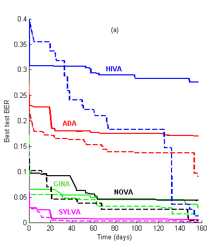
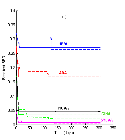
LC IJCNN06 LC IJCNN07                           Figure 1: Learning curves. We show the evolution of the best test BER as a function of time for the 2006 and the 2007 challenges, using the same datasets. (a) Performance prediction challenge. Solid lines = test set BER. Dashed lines = validation set BER (note: validation set labels were released one month before the challenge ended). (b) AL vs. PK challenge. Solid lines = AL track. Dashed lines = PK track.

For the first few weeks of the challenge, the agnostic track (AL) results kept leading (see Figure 1). The learning curves all crossed at a certain point, except for ADA. After approximately 150 days the PK performance asymptote was reached. The asymptotic performances are reported at the top of Table 2. In contrast, last year, using the same data as the AL track, the competitors attained almost their best performances in about 60 days and kept slightly improving afterwards.

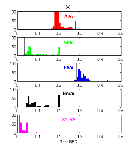
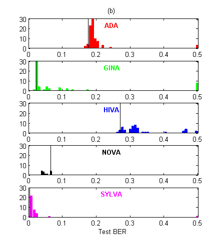
In Figure 1, we show the test BER distribution for all entries. There were about 60% more submissions in the AL track than in the PK track. This indicates that the “prior knowledge” track was harder to enter. However, the participants who did enter the PK track performed significantly better on average than those who entered the AL track, on all datasets except for HIVA. To quantify this observation we ran a Wilcoxon rank sum test on the difference between the median values of the two tracks (Table 2). We also performed paired comparisons for entrants who entered both tracks, using their last 5 submissions. In Table 2, a “+” indicates that the entrant performed best in the
PK track and a “-” indicates the opposite. We see that the entrants who entered both tracks did not always succeed in getting better results in the PK track. The pvalues of the sign test does not reveal any significant dominance of PK over AL or vice versa in that respect (all are between 0.25 and 0.5). However, for HIVA and NOVA the participants who entered both tracks failed to get better results in the PK track. We conclude that, while on average PK seems to win over AL, success is uneven and depends both on the domain and on the individuals’ expertise.


Table 2: Result statistics. The first 4 lines are computed from the test set BER over all entries, including reference entries made by the organizers. The indicate that PK wins over AL in most cases. The fifth line indicates that the median values of the 2 previous lines are significantly different (better for PK), except for HIVA. In the remainder of the table, a + indicates that in the 5 last entries of each participant having entered both tracks the best prior knowledge entry gets better results than the best agnostic entry. PK is better than AL for most entrants having entered both tracks for ADA, GINA and SYLVA, but the opposite is true for HIVA and NOVA (requiring more domain knwoledge). The last lign  tests the significance of the fraction of times PK is better than AL or vice versa (no significance found because too few participants entered both tracks).

ADA
 GINA  HIVA
NOVA
 SYLVA
Min PK BER  0.170 0.019 0.264 0.037 0.004
Min AL BER  0.166 0.033 0.271 0.046 0.006
Median PK BER  0.189 0.025 0.31 0.047 0.008
Median AL BER  0.195 0.066 0.306 0.081 0.015
Pval ranksum test 5 E-08 3 E-18 0.25 8 E-08  1 E-18
Jorge Sueiras        
Juha Reunanen    +      +
Marc Boulle  +  +  
Roman Lutz          +
Vladimir Nikulin  +      +
Vojtech Franc  +  +      
CWW      
Reference (gcc)   +  +    
Pvalue sign test  0.31 0.19 0.25 0.25 0.3

BER distribution
In Figure 2, we show the test BER distribution for all entries. There were about 60% more submissions in the AL track than in the PK track. This indicates that the “prior knowledge” track was harder to enter. However, the participants who did enter the PK track performed significantly better on average than those who entered the AL track, on all datasets except for HIVA.

Agnos Prior
Figure 2: Histograms of BER performances. The thin vertical black line indicates the best entry counting toward the final ranking (among the five last of every entrant). (a) Agnostic learning track. (b) Prior knowledge track. Note that for NOVA, the best entries are not among the last ones submitted!

To quantify this observation we ran a Wilcoxon rank sum test on the difference between the median values of the two tracks (Table 2). We also performed paired comparisons for entrants who entered both tracks, using their last 5 submissions. In Table 2, a “+” indicates that the entrant performed best in the PK track and a “-” indicates the opposite. We see that the entrants who entered both tracks did not always succeed in getting better results in the PK track. The pvalues of the sign test does not reveal any significant dominance of PK over AL or vice versa in that respect (all are between 0.25 and 0.5). However, for HIVA and NOVA the participants who entered both tracks failed to get better results in the PK track. We conclude that, while on average PK seems to win over AL, success is uneven and depends both on the domain and on the individuals’ expertise.

Result tables

Here are the final result tables as of August 1st, 2007, which determined the prizes.

Table 3: Agnostic learning track


Entrant ADA GINA HIVA NOVA SYLVA Score Ave. best
Roman Lutz 1 1 9 2 1 0.143101 LogitBoost with trees 
IDEAL, Intel 2 2 4 9 6 0.237334 out1-fs-nored-val 
Juha Reunanen 7 4 3 4 7 0.242436 cross-indexing-8 
Vladimir Nikulin 3 6 5 3 4 0.243593 vn5 
H. Jair Escalante 6 9 2 7 2 0.246381 PSMS_100_4all_NCV
Mehreen Saeed 9 5 10 1 3 0.278554 Submit D final 
Erinija Pranckeviene 10 7 6 12 10 0.435781 liknon feature selection
Joerg Wichard 8 10 8 15 8 0.481145 Final 
Namgil Lee 11 11 7 11 5 0.508458 mlp+commitee+mcic
Vojtech Franc 13 8 1 13 11 0.538075 RBF SVM 
Marc Boullé 4 13 11 5 9 0.611149 Data Grid
Zhihang Chen 15 3 16 10 12 0.64688 agnostic-resu-1 
Stijn Vanderlooy 18 14 17 17 15 0.944741 micc-ikat 


Table 4: Prior knowledge track

Entrant ADA GINA HIVA NOVA SYLVA Score Ave. best
Vladimir Nikulin 2 1 agnos agnos 3 0.0960 vn3 
Juha Reunanen agnos 3 agnos agnos 2 0.1294 cross-indexing-prior-1a
Roman Lutz agnos agnos agnos agnos 1 0.1381 Doubleboost 
Marc Boullé 1 4 agnos 2 5 0.3821 Data Grid 
Jorge Sueiras 3 5 agnos 1 4 0.3983 boost tree 
Vojtech Franc 4 2 agnos agnos agnos 0.4105 RBF SVM
Chloé Azencott (Baldi lab UCI) agnos agnos 1 agnos agnos 0.7640 SVM 

The prize winners are indicated in yellow. The best average BER is held by Reference (Gavin Cawley): try to outperform him by making post-challenge entries! Louis Duclos-Gosselin is second on ADA with Neural Network13, and S. Joshua Swamidass (Baldi Lab, UCI) second on HIVA, but they are not entered in the table because they did not submit complete entries. The overall entry ranking is performed with the overall score (average rank over all datasets, using the test BER for ranking). The best performing complete entry may not contain all the best performing entries on the individual datasets.

From the results, we noticed that it is possible to do very well without prior knowledge and using prior knowledge skillfully is not that obvious:

  •  Datasets on which PK does not seem to buy a lot: On ADA and NOVA, the best results obtained by the participants is in the agnostic track! But it is possible to do better with prior knowledge: on ADA, the PK winner did worse in the AL track; the PK best “reference” entry yields best results on NOVA.
  •  Datasets on which PK is easy to exploit: On GINA and SYLVA, significantly better results are achieved in the PK track and all but one participant who entered both tracks did better with PK. However, the kind of prior knowledge used required little domain expertise.
  •  Dataset on which PK is hard to exploit: On HIVA, experts achieve significantly better results with prior knowledge, but non-experts entering both tracks do worse in the PK track. Here domain knowledge seems to play a key role.

The most successful classification methods in this competition involve boosting algorithms or kernel-based algorithms, such as support vector machines, with the exception of the data grid models, performing well on ADA. Approaches based on the provided CLOP package are among the top ranking entries. Model selection had to be harnessed to win the contest. The challenge results indicate that conducting an effective search is critical and that simple cross-validation (CV) can be used to effectively evaluate models.

We performed intermediate rankings using the test set (but not revealing the test set performances), see Table 5:
December 1st, 2006 (for NIPS 06): Results of the model selection game. [Slides].
March 1st , 2007: Competition deadline ranking. [Slides]
The March 1st results prompted us to extend the competition deadline because the participants in the “prior knowledge track” are still making progress, as indicated by the learning curves. The best results did not significantly improve, but some entrants made significant improvements in their methods.


Table 5: Milestone results on the test set (only revealed at the end of the challenge). The letter “A” indicates the AL track and the letter “P” the PK track.
Dataset IJCNN06A NIPS06 A March07A March07P IJCNN07A IJCNN07P Best result Error bar
ADA 0.1723 0.1660 0.1660 0.1756 0.1660 0.1756 0.1660 (agnos) 0.0021
GINA 0.0288 0.0353 0.0339 0.0225 0.0339 0.0226 0.0192 (prior, ref) 0.0009
HIVA 0.2757 0.2708 0.2827 0.2741 0.2827 0.2693 0.2636 (prior, ref) 0.0068
NOVA 0.0445 0.0465 0.0463 0.0659 0.0456 0.0659 0.0367 (prior, ref) 0.0018
SYLVA 0.0661 0.0065 0.0062 0.0043 0.0062 0.0043 0.0043 (prior) 0.0004

Winning agnostic learning methods

The winner of the “agnostic learning” track is Roman Lutz, who also won the Performance Prediction Challenge (IJCNN06), using boosting techniques. Gavin Cawley, who joined the organization team and was co-winner of the previous challenge, made a reference entry using a kernel method called LSSVMs, which slightly outperforms that of Lutz. The improvements he made can partly be attributed to the introduction of an ARD kernel, which automatically downweighs the least relevant features and to a Bayesian regularization at the second level of inference. The second best entrant is the Intel group, also using boosting methods. The next best ranking entrants include Juha Reunanen and Hugo Jair Escalante, who have both been using CLOP models provided by the organizers and have proposed innovative search strategies for model selection: Escalante is using a biologically inspired particle swarm technique and Reunanen a cross-indexing method to make cross-validation more computationally efficient. Other top ranking participants in the AL track include Vladimir Nikulin and Joerg Wichard who both experimented with several ensemble methods, Erinija Pranckeviciene who performed a study of linear programming SVM methods (another kernel method), and Marc Boullé who introduced a new data grid method.

How to use prior knowledge?

We summarize the strategies employed by the participants to exploit prior knowledge on the various datasets.

ADA: the marketing application
The task of ADA is to discover high revenue people from census data, presented in the form of a two-class classification problem. The raw data from the census bureau is known as the Adult database in the UCI machine-learning repository. The 14 original attributes (features) represent age, workclass, education, education, marital status, occupation, native country, etc. and include continuous, binary and categorical features. The PK track had access to the original features and their descriptions. The AL track had access to a preprocessed numeric representation of the features, with a simple disjunctive coding of categorical variables, but the identity of the features was not revealed. We expected that the participants of the AL vs. PK challenge could gain in performance by optimizing the coding of the input features. Strategies adopted by the participants included using a thermometer code for ordinal variables (Gavin Cawley) and optimally grouping values for categorical variables (Marc Boullé). Boullé also optimally discretized continuous variables, which make them suitable for a naïve Bayes classifier. However, the advantage of using prior knowledge for ADA was marginal. The overall winner on ADA is in the agnostic track (Roman Lutz), and the entrants who entered both tracks and performed better using prior knowledge do not have results statistically significantly better. We conclude that optimally coding the variables may be not so crucial and that good performance can be obtained with a simple coding and a state-of-the-art classifier.

GINA: the handwriting recognition application

The task of GINA is handwritten digit recognition, the raw data is known as the MNIST dataset. For the “agnostic learning” track we chose the problem of separating two-digit odd numbers from two-digit even numbers. Only the unit digit is informative for this task, therefore at least 1/2 of the features are distractors. Additionally, the pixels that are almost always blank were removed and the pixel order was randomized to hide the meaning of the features. For the “prior knowledge” track, only the informative digit was provided in the original pixel map representation. In the PK track the identities of the digits (0 to 9) were provided for training, in addition to the binary target values (odd vs. even number). Since the prior knowledge track data consists of pixel maps, we expected the participants to perform image pre-processing steps such as noise filtering, smoothing, de-skewing, and feature extraction (points, loops, corners) and/or use kernels or architectures exploiting geometric invariance by small translation, rotation, and other affine transformations, which have proved to work well on this dataset. Yet, the participants to the PK track adopted very simple strategies, not involving a lot of domain knowledge. Some just relied on the performance boost obtained by the removal of the distractor features (Vladimir Nikulin, Marc Boullé, Juha Reunanen). Others exploited the knowledge of the individual class labels and created multi-class of hierarchical classifiers (Vojtech Franc, Gavin Cawley). Only the reference entries of Gavin Cawley (which obtained the best BER of 0.0192) included domain knowledge by using an RBF kernels with tunable receptive fields to smooth the pixel maps. In the future, it would be interesting to assess the methods of Simard et al on this data to see whether further improvements are obtained by exploiting geometrical invariances. The agnostic track data was significantly harder to analyze because of the hidden class heterogeneity and the presence of feature distractors. The best GINA final entry was therefore on the PK track and all four ranked entrants who entered both tracks obtained better results in the PK track. Further, the differences in performance are all statistically significant.

HIVA: the drug discovery application
The task of HIVA is to predict which compounds are active against the AIDS HIV infection. The original data from the NCI has 3 classes (active, moderately active, and inactive). We brought it back to a two-class classification problem (active & moderately active vs. inactive), but we provided the original labels for the “prior knowledge” track. The compounds are represented by their 3d molecular structure for the “prior knowledge” track (in SD format). For the “agnostic track” we represented the input data as vector of 2000 sparse binary variables. The variables represent properties of the molecule inferred from its structure by the ChemTK software package (version 4.1.1, Sage Informatics LLC). The problem is therefore to relate structure to activity (a QSAR – quantitative structure-activity relationship problem) to screen new compounds before actually testing them (a HTS – high-throughput screening problem). Note that in such applications the BER is not the best metric to assess performances since the real goal is to identify correctly the compounds most likely to be effective (belonging to the positive class). We resorted to using the BER to make comparisons easier across datasets. The raw data was not supplied in a convenient feature representation, which made it impossible to enter the PK track using agnostic learning methods, using off-the-shelf machine learning packages. The winner in HIVA (Chloé-Agathe Azencott of the Pierre Baldi Laboratory at UCI) is a specialist in this kind of dataset, on which she is working towards her PhD. She devised her own set of low level features, yielding a “molecular fingerprint” representation, which outperformed the ChemTK features used on the agnostic track. Her winning entry has a test BER of 0.2693, which is significantly better than the test BER of the best ranked AL entry of 0.2827 (error bar 0.0068). The results on HIVA are quite interesting because most agnostic learning entrants did not even attempt to enter the prior knowledge track and the entrants that did submit models for both tracks failed to obtain better results in the PK track. One of them working in an institute of pharmacology reported that too much domain knowledge is sometimes detrimental; experts in his institute advised against using molecular fingerprints, which ended up as the winning technique.

NOVA: the text classification application
The data of NOVA come from the 20-Newsgroup dataset. Each text to classify represents a message that was posted to one or several USENET newsgroups. The raw data is provided in the form of text files for the “prior knowledge” track. The preprocessed data for the “agnostic learning” track is a sparse binary representation using a bag-of-words with a vocabulary of approximately 17000 words (the features are simply frequencies of words in text). The original task is a 20-class classification problem but we grouped the classes into two categories (politics and religion vs. others) to make it a two-class problem. The original class labels were available for training in the PK track but not in the AL track. As the raw data consist of texts of variable length it was not possible to enter the PK track for NOVA without performing a significant pre-processing. All PK entrants in the NOVA track used a bag-ofwords representation, similar to the one provided in the agnostic track. Standard tricks were used, including stemming. Gavin Cawley used the additional idea of correcting the emails with an automated spell checker and Jorge Sueiras used a Thesaurus. No entrant who entered both tracks outperformed their AL entry with their PK entry in their last ranked entries, including the winner! This is interesting because the best PK entries made throughout the challenge significantly outperform the best AL entries (BER difference of 0.0089 for an error bar of 0.0018), see also Figure 1. Hence in this case, the PK entrants overfitted and were unable to select among their PK entries those, which would perform best on test data. This is not so surprising because the validation set on NOVA is quite small (175 examples). Even though the bag-of-words representation is known to be state-of-the-art for this kind of applications, it would be interesting to compare it with more sophisticated representations. To our knowledge, the best results on the 20 Newsgroup data were obtained by the method of distributional clustering by Ron Bekkerman.

SYLVA: the ecology application
The task of SYLVA is to classify forest cover types. The forest cover type for 30 x 30 meter cells was obtained from US Forest Service (USFS) Region 2 Resource Information System (RIS) data. We converted this into a two-class classification problem (classifying Ponderosa pine vs. everything else). The input vector for the “agnostic learning“ track consists of 216 input variables. Each pattern is composed of 4 records: 2 true records matching the target and 2 records picked at random. Thus 1/2 of the features are distractors. The “prior knowledge” track data is identical to the “agnostic learning” track data, except that the distractors are removed and the meaning of the features is revealed. For that track, the identifiers in the original forest cover dataset are revealed for the training set. As the raw data was already in a feature vector representation, this task was essentially testing the ability of the participants in the AL track to perform well in the presence of distractor features. The PK track winner (Roman Lutz) in his Doubleboost algorithm exploited the fact that each pattern was made of two records of the same pattern to train a classifier with twice as many training examples. Specifically, a new dataset was constructed by putting the second half of the data (variables 55 to 108) below the first half (variables 1 to 54). The new dataset is of dimension 2n times 54 (instead of n times 108). This new dataset is used for fitting the base learner (tree) of his boosting algorithm. The output of the base learner is averaged over the two records belonging to the same pattern. This strategy can be related to the neural network architectures using “shared weights”, whereby at training time, the weights trained on parts of the pattern having similar properties are constrained to be identical. This reduced the number of free parameters of the classifier.

Conclusions

For the first few month of the challenge, AL lead over PK, showing that the development of good AL classifiers is considerably faster. As of March 1st 2007, PK was leading over AL on four out of five datasets. We extended the challenge five more month, but the best performances did not significant improve during that time period. On datasets not requiring real expert domain knowledge (ADA, GINA, SYLVA), the participants entering both track obtained better results in the PK track, using a special-purpose coding of the inputs and/or the outputs, exploiting the knowledge of which features were uninformative, and using “shared weights” for redundantfeatures. For two datasets (HIVA and NOVA) the raw data was not in a feature representation and required some domain knowledge to preprocess data. The winning data representations consist in low level features (“molecular fingerprints” and “bag of words”). From the analysis of this challenge, we conclude that agnostic learning methods are very powerful. They quickly yield (in 40 to 60 days) to performances, which are near the best achievable performances. General-purpose techniques for exploiting prior knowledge in the encoding of inputs or outputs or the design of the learning machine architecture (e.g. via shared weights) may provide an additional performance boost, but exploiting real domain knowledge is both hard and time consuming. The net result of using domain knowledge rather using than low level features and relying on agnostic learning may actually be to worsen results, as experienced by some entrants. This fact seems to be a recurrent theme in machine learning publications and the results of our challenge confirm it. Future work includes incorporating the best identified methods in our challenge toolkit CLOP. The challenge web site remains open for post-challenge submissions.


Description

The goal of the challenge is to identify the different Machine Learning (ML) methods proposed so far for structured data, to assess the potential of these methods for dealing with generic ML tasks in the structured domain, to identify the new challenges of this emerging field and to foster research in this domain. Structured data appears in many different domains. We will focus here on Graph document collections and we are organizing this challenge in cooperation with the INEX initiative. This challenge aims at gathering ML, Information Retrieval (IR) and Data Mining researchers in order to:

  • Define the new challenges for structured data mining with ML techniques.
  • Build Interlinked document collections, define evaluation methodologies and develop software which will be used for the evaluation of classification of documents in a graph.
  • Compare existing methods on different datasets.

Results of the track will be presented at the INEX workshop.

 Task : Graph (Semi-)Supervised Classification

Dealing with XML document collections is a particularly challenging task for ML and IR. XML documents are de¯ned by their logical structure and their content (hence the name semi-structured data). Moreover, in a large majority of cases (Web collections for example), XML documents collections are also structured by links between documents (hyperlinks for example). These links can be of different types and correspond to different nformation: for example, one collection can provide hierarchical links, hyperlinks, citations, etc.

Earlier models developed in the field of XML categorization/clustering simultaneously use the content information and the internal structure of XML documents for a list of models) but they rarely use the external structure of the collection i.e the links between documents.

We focus here on the problem of classication of XML documents organized in graph. More precisely, the participants of the task have to classify the document of a partially labelled graph.

Tasks

Collection

The corpus used this year will be a subset of the Wikipedia XML Corpus of INEX 2009. This subset will be different than the one used last year. Mainly:

  • Each document will belong to one or more than one categories
  • Each document will be and XML document
  • The different documents will be organized in a graph of documents where each link correspond to an hyperlink (or wiki link) between two documents

The corpus proposed is a graph of XML documents.

Semi supervised classification

In this track, the goal is to classify each node of a graph (a node corresponds to a document) knowing a set of already labelled nodes (the training documents). In the ML point of view, the track proposed here is a transductive (or semi) supervised classification task.

The following figure gives an example of classification task.

Training set: The training set is composed of XML documents organized in a graph. The red nodes correspond to documents in category 1, the blue nodes corresponds to documents in category 2. The white nodes correspond to documents where the category is hidden. The goal of the categorization task is to find the categories of the white nodes
The goal of the categorization models are to find the color of the unlabelled nodes of the training graph.

The evaluation measure for categorization will be ROC curves and F1 measure

Results by team

The measures computed are:

Package for computing performances

In order to use the package, you have to write:

 perl compute.pl all_categories.txt train_categories.txt yourSubmissionFile

If the software find negative scores in the file, it normalizes the score by applying a logistic function over the scores.

Introduction

Touch Clarity (www.touchclarity.com) provides real­time optimisation of websites. Touch Clarity chooses, from a number of options, the most popular content to display on a page. This decision is made by tracking how many visitors respond to each of the options, by clicking on them. This is a direct commercial application of the multi­armed bandit problem – each of the items which might be shown is a separate bandit, with a separate response rate.

As in the multi­armed bandit problem, there is a trade­off between exploration and exploitation – it is necessary to sometimes serve items other than the most popular in order to measure their response rate with sufficient precision to correctly identify which is the most popular. However, in this application there is a further complication – typically the rates of response to each item will vary over time, so continuous exploration is necessary in order to track this time variation, as old knowledge becomes out ­of­ date. An extreme example of this might be in choosing which news story to serve as the main story on a news page – interest in one story will decrease over time while interest in another will increase. In addition, the interest in several stories might vary in a similar, coherent way – for example a general increase in interest in sports stories at weekends, or in political stories near to an election. So there are typically two types of variation to consider – where response rates vary together, and where response rates vary completely independently.

The Challenge

The challenge aims to stimulate research into the optimal way to trade­off exploration vs exploitation where the response rate for each option is varying over time. Instead of a static data set, data for the challenge is provided in the form of a visitor behaviour simulation engine, written in java, and also made available as a Matlab function.

Entrants should write a program which will repeatedly choose from a range of possible display options, and query the visitor simulation engine through an interface e.g.

public Boolean selectOption(int option)The engine will return true or false, depending on whether the simulated visitor responded to the option that was served to them. The objective is to maximize the number of positive responses returned by the engine. The response rate for each option varies over time. The visitor simulation engine maintains time ­dependent continuous functions for the response rate of each of the options. When the engine is queried with a given option, it calculates the value of the function at that time. The engine returns true with a probability given by this value. The time variable used is the number of requests made to the engine, rather than real time. This is to remove dependencies on the machine hardware, and application performance of the entrants. In this application there is no fixed horizon, that is to say the number of trials is not fixed, and so solutions should not use the number of trials as a parameter.

To prevent the engine from repeating the same behaviour every time it is restarted, the response rate functions are parameterized. On restart, new values for these parameters are randomly generated based on a seed.

The challenge is broken into a number of individual tasks each relating to a particular problem that is frequently encountered in real website data. The engine addresses each of these problems in turn.

Tasks

There are now six tasks, the old tasks are now invalid. In each task there are 5 options. The best achievable response rate is approximately 0.18 for all tasks. All tasks are designed to display the appropriate behaviour over 1M requests. (Although during the judging phase more may be required.)

Task 1. SimulatedVisitorFrequentSwap

To check a candidate algorithm can respond to relatively frequent changes of the best option.

Task 2. SimulatedVisitorLongGaussians

To check a candidate algorithm can respond to changes of the best option over longer time periods.

Task 3. SimulatedVisitorWeeklyVariation

To check a candidate algorithm can handle coherent variation of response rates where there are two sinusoidal components to the variation of differing periods, the longer period being dominant. In addition, there is a gradual change in the relative ranking of the option. This is to ensure there is ongoing exploration throughout the run and that it can handle the consequent comparison of option response rates that have been served at different times. In addition, each option has a randomly chosen start time.

Task 4. SimulatedVisitorDailyVariation

To check a candidate algorithm can handle coherent variation of response rates where there are two sinusoidal components to the variation of differing periods, the shorter period being dominant.

Task 5. SimulatedVisitorWeeklyCloseVariation

To check a candidate algorithm can handle coherent variation where response rates are closely spaced.

Task 6. SimulatedVisitorConstant

We must ensure a candidate algorithm can handle the ideal case. An over exploratory algorithm can degrade to random performance under these conditions.

Organisers

Zakria Hussain, University College, London
Peter Auer, University of Leoben
Nicolò Cesa-Bianchi, Università degli Studi di Milano
Leonard Newnham, Touch Clarity
John Shawe-Taylor, University College, London

Submission of Results

Results can be submitted at any time via the submit tab, a set of random seeds is available here. Run your code using these seeds with each run of length 1M requests.

Judging

During the judging phase of the challenge, a further evaluation will take place for each algorithm. This is to ensure candidate algorithms can perform well over a variety of conditions. A second set of random seeds will be published along with a different run length. Each entrant will be re-evaluated against these seeds and run length. The winner of the challenge will be the entrant who obtains the lowest total regret on all six tasks. There is no longer the option of submitting for one task only.

Touch Clarity reserves the right to disqualify entrants if any of the following rules are broken:

  • No algorithm should use the run length as an input parameter. In a real application optimisation does not terminate after a particular number of requests.
  • Algorithms should NOT use information about the shape of the response functions obtained during the course of a run. The response function information available from the csv files is to assist in improving the performance of algorithms only. The sort of solution we are trying to avoid is “if resp rates constant over first 1000 responses then use USB otherwise use SomeOtherAlgorithm”.


Java code download

Java-code1.2.zip (version 1.2 released 21st May 2006)

There is an API written in Java which is distributed as a .jar file (.class executables only) and some baseline Java code that implements some simple multi-armed bandit problem algorithms. You will need at least Java version 1.5 to run the Java code. You can compile the baseline code like so:

javac -classpath challenge1.2.jar applicationtest/*.java applicationtest/simplewindowprovider/*.java

After this you can run ApplicationTest like so:

java -classpath .;challenge1.2.jar -Xmx256m applicationtest/ApplicationTest

OR

java -classpath :challenge1.2.jar -Xmx256m applicationtest/ApplicationTest

The Java code contains provider classes and several (bandit) algorithms written using the provider classes. ApplicationTest calls these algorithms and runs them on all 6 tasks. All participants will need to write their algorithm as a provider class. Please look at the provider classes in the sample Java code to understand how to do this. The code contains very simplistic algorithms for bandit problems when arms do not vary over time. However, please note that the challenge is for the case where the rewards for an arm varies over time.

Version 1.1 contains:

      1. Six new tasks
      2. detailed output every 1000 requests to csv file. This contains:
        1. the underlying response rates of the options in the task, and
        2. the proportion of serves each option is receiving

This allows the user to construct clear graphical views of how an algorithm is performing over time – see for example

UCBWindowProvider.JPG

    .

  1. An efficiency metric has been added to getStatistics(). This ranges from 0 (equivalent to random serving) to 1 (equalling the maximum theoretical success rate).

Version 1.2 contains

  1. UCBWindowProvider – a windowed version of UCB
  2. Improved regret summary
  3. improved commandline args:
    1. -h help
    2. -r number of requests
    3. -s random seed set
    4. -i produce results on interim seed set. The summary printed at the end of the test is sufficient for a submission
  4. better javadoc of applicationtest and challenge1.2.jar

Here is the javadoc1.2 for the challenge1.2.jar package.

Matlab code download

Matlab-code1.2.zip (version 1.2 released 21st May 2006)

The Matlab code is a wrapper for the Java API but does not contain any baseline code like that available for the Java download. The Matlab wrapper calls in the challenge1.2.jar executables and all its functions can be used as in Java. Please read the documentation (preamble) in the matlab file in order to set it up to run correctly.


Results of Phase 2 tasks

THE WINNING ALGORITHM WILL BE THE ONE THAT IS RANKED NUMBER 1 IN THE “TOTAL AVERAGE REGRET FOR TASKS 1-6” TABLE USING THE TEST SEEDS.

Total Average Regret for tasks 1-6

Rank
Algorithm
Name
Institution
Total Average Regret
Validation Seeds
Test Seeds
1
MetaUCBFC Nicolas Baskiotis, Cedric Hartland & Sylvain Gelly Univ Paris XI Orsay – lri 34599.203 34202.5
2
ProviderDiscountedUCB Thomas Jaksch University of Leoben 35071.0 36073.797
3
ProviderExp4DWrapper Thomas Jaksch University of Leoben 35120.0 36253.9
4
UCB1DiscountTuned Flóra Adorján & György Ottucsák Budapest University of Technology and Economics 37066.2 37117.8
5
MetaUCB Nicolas Baskiotis, Cedric Hartland & Sylvain Gelly Univ Paris XI Orsay – lri 35532.4 37282.203
6
UCB1DiscountTuned_C Flóra Adorján & György Ottucsák Budapest University of Technology and Economics 36948.3 37744.7
7
UCB1DiscountTuned_B Flóra Adorján & György Ottucsák Budapest University of Technology and Economics 37356.2 38194.6
8
TaoUcbForgetPascalChallenge Nicolas Baskiotis, Cedric Hartland & Sylvain Gelly Univ Paris XI Orsay – lri 39605.4 43969.7
9
UCBWindowProvider Baseline code 180301.81 179246.31
10
ShiftingBanditProvider Baseline code 211875.2 211107.8
11
ProviderUCB Baseline code 222884.5 249174.6
12
RandomProvider Baseline code 322342.7 318739.6


Task 1. SimulatedVisitorFrequentSwap

Rank
Algorithm
Name
Institution
Validation Seeds
Test Seeds
Average Regret
STD
Average Regret
STD
1
ProviderExp4DWrapper Thomas Jaksch University of Leoben 9183.5 614.5174 9133.0 508.81235
2
MetaUCBFC Nicolas Baskiotis, Cedric Hartland & Sylvain Gelly Univ Paris XI Orsay – lri 11052.9 1126.048 9906.5 780.7754
3
ProviderDiscountedUCB Thomas Jaksch University of Leoben 10198.4 933.2443 10697.9 1380.2686
4
UCB1DiscountTuned_C Flóra Adorján & György Ottucsák Budapest University of Technology and Economics 12059.8 884.5122 11983.7 618.63525
5
TaoUcbForgetPascalChallenge Nicolas Baskiotis, Cedric Hartland & Sylvain Gelly Univ Paris XI Orsay – lri 12036.0 658.0817 12057.5 879.0806
6
UCB1DiscountTuned_B Flóra Adorján & György Ottucsák Budapest University of Technology and Economics 11992.7 618.4238 12303.9 546.7468
7
UCB1DiscountTuned Flóra Adorján & György Ottucsák Budapest University of Technology and Economics 12152.8 701.47064 12330.8 766.26135
8
MetaUCB Nicolas Baskiotis, Cedric Hartland & Sylvain Gelly Univ Paris XI Orsay – lri 15298.1 1714.1592 15265.4 3004.444
9
ProviderUCB Baseline code 32832.0 942.6005 32392.5 828.2142
10
UCBWindowProvider Baseline code 36098.6 1702.405 35564.0 1964.2234
11
ShiftingBanditProvider Baseline code 40806.8 1312.9364 40947.7 1463.947
12
RandomProvider Baseline code 48835.7 460.32596 49054.1 503.07773


Task 2. SimulatedVisitorLongGaussians

Rank
Algorithm
Name
Institution
Validation Seeds
Test Seeds
Average Regret
STD
Average Regret
STD
1
ProviderDiscountedUCB Thomas Jaksch University of Leoben 3032.5 467.23615 3350.2 451.85638
2
UCB1DiscountTuned_C Flóra Adorján & György Ottucsák Budapest University of Technology and Economics 3854.6 393.24185 4020.2 678.94574
3
UCB1DiscountTuned_B Flóra Adorján & György Ottucsák Budapest University of Technology and Economics 3877.9 328.87567 4031.0 400.47943
4
UCB1DiscountTuned Flóra Adorján & György Ottucsák Budapest University of Technology and Economics 3819.4 331.3753 4133.9 631.6608
5
MetaUCBFC Nicolas Baskiotis, Cedric Hartland & Sylvain Gelly Univ Paris XI Orsay – lri 4550.2 1560.2434 4561.1 975.12006
6
ProviderExp4DWrapper Thomas Jaksch University of Leoben 4767.9 389.79468 4622.5 283.90424
7
MetaUCB Nicolas Baskiotis, Cedric Hartland & Sylvain Gelly Univ Paris XI Orsay – lri 4817.5 1670.4481 5636.5 1254.3213
8
TaoUcbForgetPascalChallenge Nicolas Baskiotis, Cedric Hartland & Sylvain Gelly Univ Paris XI Orsay – lri 7352.9 2036.1892 8613.9 1643.2212
9
ShiftingBanditsProvider Baseline code 47240.3 3023.0012 46586.8 3428.574
10
ProviderUCB Baseline code 51547.9 10747.207 68992.3 29760.65
11
UCBWindowProvider Baseline code 64994.6 14387.951 69414.7 25192.545
12
RandomProvider Baseline code 113337.1 7096.978 109707.5 7496.9795

Task 3. SimulatedVisitorWeeklyVariation

Rank
Algorithm
Name
Institution
Validation Seeds
Test Seeds
Average Regret
STD
Average Regret
STD
1
ProviderDiscountedUCB Thomas Jaksch University of Leoben 3947.0 559.38635 3651.8 393.22647
2
UCB1DiscountTuned Flóra Adorján & György Ottucsák Budapest University of Technology and Economics 4385.6 545.81683 4451.5 523.6664
3
UCB1DiscountTuned_B Flóra Adorján & György Ottucsák Budapest University of Technology and Economics 4647.5 515.3112 4533.6 249.49202
4
MetaUCB Nicolas Baskiotis, Cedric Hartland & Sylvain Gelly Univ Paris XI Orsay – lri 4534.5 723.832 4558.7 735.7625
5
UCB1DiscountTuned_C Flóra Adorján & György Ottucsák Budapest University of Technology and Economics 4486.4 463.7919 4676.3 703.2815
6
MetaUCBFC Nicolas Baskiotis, Cedric Hartland & Sylvain Gelly Univ Paris XI Orsay – lri 4764.3 556.171 5213.6 541.3687
7
ProviderExp4DWrapper Thomas Jaksch University of Leoben 7511.4 1893.0953 7999.3 673.5912
8
TaoUcbForgetPascalChallenge Nicolas Baskiotis, Cedric Hartland & Sylvain Gelly Univ Paris XI Orsay – lri 7084.7 950.5174 8206.8 787.7223
9
UCBWindowProvider Baseline code 29055.3 11124.4 21102.5 12444.306
10
ShiftingBanditsProvider Baseline code 40649.8 212.50716 40609.1 220.46388
11
RandomProvider Baseline code 57238.3 308.08838 57185.8 253.00189
12
ProviderUCB Baseline code 61824.0 2355.0454 63349.5 934.28564


Task 4. SimulatedVisitorDailyVariation

Rank
Algorithm
Name
Institution
Validation Seeds
Test Seeds
Average Regret
STD
Average Regret
STD
1
UCB1DiscountTuned_B Flóra Adorján & György Ottucsák Budapest University of Technology and Economics 4728.9 883.0477 5070.2 947.57245
2
UCB1DiscountTuned Flóra Adorján & György Ottucsák Budapest University of Technology and Economics 5751.8 1262.6565 5097.0 1017.7952
3
ProviderExp4DWrapper Thomas Jaksch University of Leoben 4884.9 492.63092 5140.2 365.1742
4
UCB1DiscountTuned_C Flóra Adorján & György Ottucsák Budapest University of Technology and Economics 4751.9 1495.7024 5253.9 1112.1284
5
MetaUCBFC Nicolas Baskiotis, Cedric Hartland & Sylvain Gelly Univ Paris XI Orsay – lri 5870.1 617.5396 6179.0 697.5103
6
MetaUCB Nicolas Baskiotis, Cedric Hartland & Sylvain Gelly Univ Paris XI Orsay – lri 5657.9 712.6532 6188.6 1034.8442
7
TaoUcbForgetPascalChallenge Nicolas Baskiotis, Cedric Hartland & Sylvain Gelly Univ Paris XI Orsay – lri 5946.6 786.82513 7897.1 4283.818
8
ProviderDiscountedUCB Thomas Jaksch University of Leoben 7253.1 774.3874 8043.3 1215.4939
9
UCBWindowProvider Baseline code 30567.3 17000.268 34363.6 19650.63
10
ShiftingBanditsProvider Baseline code 42619.6 205.62112 42662.3 194.08247
11
RandomProvider Baseline code 57109.8 238.72942 57112.7 220.19237
12
ProviderUCB Baseline code 54405.2 9520.59 61281.9 6575.8525


Task 5. SimulatedVisitorWeeklyCloseVariation

Rank
Algorithm
Name
Institution
Validation Seeds
Test Seeds
Average Regret
STD
Average Regret
STD
1
UCB1DiscountTuned Flóra Adorján & György Ottucsák Budapest University of Technology and Economics 4947.8 375.51675 4981.1 498.89618
2
ProviderDiscountedUCB Thomas Jaksch University of Leoben 5137.5 466.3166 5052.9 450.37573
3
MetaUCB Nicolas Baskiotis, Cedric Hartland & Sylvain Gelly Univ Paris XI Orsay – lri 4656.4 555.3968 5088.1 739.60144
4
MetaUCBFC Nicolas Baskiotis, Cedric Hartland & Sylvain Gelly Univ Paris XI Orsay – lri 5280.0 654.064 5162.6 756.14844
5
UCB1DiscountTuned_C Flóra Adorján & György Ottucsák Budapest University of Technology and Economics 5440.7 326.4149 5243.8 421.37152
6
UCB1DiscountTuned_B Flóra Adorján & György Ottucsák Budapest University of Technology and Economics 5584.6 286.54074 5634.7 401.08328
7
TaoUcbForgetPascalChallenge Nicolas Baskiotis, Cedric Hartland & Sylvain Gelly Univ Paris XI Orsay – lri 6813.1 804.2061 6722.4 845.91504
8
ProviderExp4DWrapper Thomas Jaksch University of Leoben 7119.8 1833.6073 7557.7 1736.7368
9
UCBWindowProvider Baseline code 15240.1 2971.088 14502.9 4624.025
10
ShiftingBanditsProvider Baseline code 21690.1 364.62173 21514.2 245.27754
11
ProviderUCB Baseline code 21909.6 2055.3625 22709.6 3313.902
12
RandomProvider Baseline code 25764.2 339.47043 25654.9 343.23346


Task 6. SimulatedVisitorConstant

Rank
Algorithm
Name
Institution
Validation Seeds
Test Seeds
Average Regret
STD
Average Regret
STD
1
ProviderUCB Baseline code 365.8 74.90705 448.8 128.11522
2
TaoUcbForgetPascalChallenge Nicolas Baskiotis, Cedric Hartland & Sylvain Gelly Univ Paris XI Orsay – lri 372.1 82.51525 472.0 142.9662
3
MetaUCB Nicolas Baskiotis, Cedric Hartland & Sylvain Gelly Univ Paris XI Orsay – lri 568.0 313.2266 544.9 257.33353
4
ProviderExp4DWrapper Thomas Jaksch University of Leoben 1652.5 228.85185 1801.2 176.14943
5
MetaUCBFC Nicolas Baskiotis, Cedric Hartland & Sylvain Gelly Univ Paris XI Orsay – lri 3081.7 170.6159 3179.7 340.06668
6
UCBWindowProvider Baseline code 4345.9 250.39633 4298.6 278.8549
7
ProviderDiscountedUCB Thomas Jaksch University of Leoben 5502.5 491.91965 5277.7 426.59714
8
UCB1DiscountTuned Flóra Adorján & György Ottucsák Budapest University of Technology and Economics 6008.8 453.98135 6123.5 396.33356
9
UCB1DiscountTuned_C Flóra Adorján & György Ottucsák Budapest University of Technology and Economics 6354.9 437.75983 6566.8 449.95624
10
UCB1DiscountTuned_B Flóra Adorján & György Ottucsák Budapest University of Technology and Economics 6524.6 347.51184 6621.2 335.8319
11
ShiftingBanditProvider Baseline code 18868.6 104.250984 18787.7 135.26276
12
RandomProvider Baseline code 20057.6 104.72313 20024.6 152.13971

Old Phase 1 tasks

These are the old tasks from phase 1 and are no longer used for phase 2.

Task 1

Rank Algorithm Name Institution STD Average Regret
1 UCBg Levente Kocsis mta sztaki 34.7 52.1
2 ProviderUCB (Baseline) 24.28 65.6
3 Mean/variance regret Craig Saunders University of Southampton 61.28 89.3
4 ShiftingBanditProvider (Baseline) 21.58 141.2
5 RandomProvider (Baseline) 25.42 151.4

Task 2

Rank Algorithm Name Institution STD Average Regret
1 UCBgper Levente Kocsis mta sztaki 803.1 627.4
2 ShiftingBanditsProvider (Baseline) 206.53 1839.3
3 Stupid Switcher Craig Saunders University of Southampton 334.27 3669.3
4 Experts Prediction Cedric Hartland Laboratoire de Recherche en Informatique 1283.36 6318.6
5 ProviderUCB (Baseline) 4045.41 13270.7
6 UCBW Levente Kocsis mta sztaki 2298.62 18430.1
7 UCBg Levente Kocsis mta sztaki 8367.2 23552.7
8 RandomProvider (Baseline) 3153.57 27434.2

Task 3

Rank Algorithm Name Institution STD Average Regret
1 Mean/variance regret Craig Saunders University of Southampton 4.95 10.3
2 UCBS Levente Kocsis mta sztaki 10.39 15.3
3 UCBg Levente Kocsis mta sztaki 17.03 26.3
4 ProviderUCB (Baseline) 11.85 80.7
5 ShiftingBanditsProvider (Baseline) 40.24 765.2
6 RandomProvider (Baseline) 41.14 892.5

Development Kit

The development kit provided for the VOC challenge 2006 is available. You can:

Datasets

Following completion of the challenge, the training/validation sets with complete annotation have now been made available on the database page. Some additional example images are online.

The VOC2006 data includes some images provided by Microsoft Research Cambridge and “flickr”. Use of these images must respect the corresponding terms of use:

Details of the contributor of each image can be found in the file “contrib.txt” included in the dataset. Any queries about the use or ownership of the data should be addressed to the organizers.

Second Round

The second round aims to give an opportunity for groups who participated to submit additional results, and for others who might have been unable to meet the first deadline to participate. The deadline for submission of results for the second round is 11pm GMT, Friday 30th June 2006.

The second round will be run as per the first round. In evaluating the second round, submitted results will be evaluated separately from the first round to give consideration for the additional time available. Comparison of the results obtained between the first and second rounds will follow. As in the first round, ground truth annotation will not be provided for the test data.

On completion of the second round, the test set annotation will be released for researchers wishing to use the data for further evaluation.

Post-Challenge Submissions

We invite submission of results obtained after the completion of the challenge, both by participants and those who did not participate in the challenge. Results will be treated as distinct from the results obtained during the challenge due to the availability of the test data annotation. If you would like your results included in the online summary of results, please contact Mark Everingham, me@comp.leeds.ac.uk.

Results

A technical report summarizing the challenge and results is now available. The results may also be browsed online. Slides presented at the challenge workshop can also be downloaded.

If you make use of the VOC2006 data, please cite the following reference in any publications:

    @misc{pascal-voc-2006,
      author = "Everingham, M. and Zisserman, A. and Williams, C. K. I. and Van~Gool, L.",
      title = "The {PASCAL} {V}isual {O}bject {C}lasses {C}hallenge 2006 {(VOC2006)} {R}esults",
      howpublished = "http://www.pascal-network.org/challenges/VOC/voc2006/results.pdf"
    }

Timetable

  • 14 Feb 2006 : Development kit (training and validation data plus evaluation software) made available.
  • 31 March 2006: Test set made available.
  • 25 April 2006, 11pm GMT: DEADLINE for submission of results. There will be no further extensions.
  • 7 May 2006: Challenge workshop to be held in conjunction with ECCV06, Graz, Austria. The programme is now online.
  • 30 June 2006, 11pm GMT: DEADLINE for submission of second round results.
  • After 1 July 2006: Test set annotation made available.

Introduction

The goal of this challenge is to recognize objects from a number of visual object classes in realistic scenes (i.e. not pre-segmented objects). It is fundamentally a supervised learning learning problem in that a training set of labelled images is provided. The ten object classes that have been selected are:

  • bicycle, bus, car, motorbike
  • cat, cow, dog, horse, sheep
  • person

There will be two main competitions:

  1. For each of the ten classes, predicting presence/absence of an example of that class in the test image.
  2. Predicting the bounding box and label of each object from the ten target classes in the test image.

Participants may enter either (or both) of these competitions, and can choose to tackle any (or all) of the ten object classes. The challenge allows for two approaches to each of the competitions:

  1. Participants may use systems built or trained using any methods or data excluding the provided test sets.
  2. Systems are to be built or trained using only the provided training data.

The intention in the first case is to establish just what level of success can currently be achieved on these problems and by what method; in the second case the intention is to establish which method is most successful given a specified training set.

Data

The training data provided consists of a set of images; each image has an annotation file giving a bounding box and object class label for each object in one of the ten classes present in the image. Note that multiple objects from multiple classes may be present in the same image. Some example images can be viewed online.

Annotation was performed according to a set of guidelines distributed to all annotators. These guidelines can be viewed here.

The data will be made available in two stages; in the first stage, a development kit will be released consisting of training and validation data, plus evaluation software (written in MATLAB). One purpose of the validation set is to demonstrate how the evaluation software works ahead of the competition submission.

In the second stage, the test set will be made available for the actual competition. In contrast to the 2005 VOC challenge, no ground truth for the test data will be released until after the challenge is complete.

Following completion of the challenge, the training/validation sets with complete annotation have now been made available on the database page.

The table below summarizes statistics of the training/validation and test data. The data has been split into 50% for training/validation and 50% for testing. The distributions of images and objects by class are approximately equal across the training/validation and test sets. In total there are 5304 images, containing 9507 annotated objects.

train val trainval test
Images Objects Images Objects Images Objects Images Objects
Bicycle 127 161 143 162 270 323 268 326
Bus 93 118 81 117 174 235 180 233
Car 271 427 282 427 553 854 544 854
Cat 192 214 194 215 386 429 388 429
Cow 102 156 104 157 206 313 197 315
Dog 189 211 176 211 365 422 370 423
Horse 129 164 118 162 247 326 254 324
Motorbike 118 138 117 137 235 275 234 274
Person 319 577 347 579 666 1156 675 1153
Sheep 119 211 132 210 251 421 238 422
Total 1277 2377 1341 2377 2618 4754 2686 4753

Database Rights

The VOC2006 data includes some images provided by Microsoft Research Cambridge and “flickr”. Use of these images must respect the corresponding terms of use:

For the purposes of the challenge, the identity of the images in the database, e.g. source and name of owner, was obscured. Details of the contributor of each image can be found in the file “contrib.txt” in the final release of the data. Any queries about the use or ownership of the data should be addressed to the organizers.

Submission of Results

Participants are expected to submit a single set of results per method employed. Participants who have investigated several algorithms may submit one result per method. Changes in algorithm parameters do not constitute a different method – all parameter tuning must be conducted using the training and validation data alone.

Details of the required file formats for submitted results can be found in the development kit documentation. For each competition you should produce a single text file, named following the examples in the development kit. For example, your results file for competition 1 (classification trained on VOC data) on the “car” class should be named “comp1_cls_test_car.txt”; your results file for competition 4 (detection trained on your own data) on the “car” class should be named “comp4_det_test_car.txt”.

If you intend to submit results for several different methods, please place results for each in a separate, clearly named directory. For each method you submit, please include a brief description of the approach used. If you wish to withhold details of the method, e.g. for commercial reasons, please make this clear. Methods submitted without a description will be judged in a separate category of the challenge.

The results files should be collected in a single archive file (tar/zip) and placed on an FTP/HTTP server accessible from outside your institution. Email the URL and any details needed to access the file to Mark Everingham, me@comp.leeds.ac.uk. Please do not send files directly by email.

Publication Policy

The main mechanism for dissemination of the results will be the challenge webpage. It is also possible that an overview paper of the results will be produced.

If you make use of the VOC2006 data, please cite the technical report of results, see the results section.

Organizers

  • Mark Everingham (Oxford/Leeds), me@comp.leeds.ox.ac.uk
  • Luc van Gool (Zurich)
  • Chris Williams (Edinburgh)
  • Andrew Zisserman (Oxford)

Challenge description

There are two main goals for this challenge:

  • to test and compare different text visualization methods, ideas and algorithms on a common data-set, and
  • to contribute to the Pascal dissemination and promotion activities by using data about scientific publications from Pascal’s EPrints server.

The challenge is split into two parts where the task in the first round is very general. A more precise task, together with precise evaluation criterias, will be decided at the workshop in Venice, based on the submissions and ideas from the first round.

The data is available in the raw ePrints format. Besides it we offer a preprocessed version of the raw data into many standard formats. We also processed the data into a “baseline” visualization which can be viewed with the Document Atlas software. In this way we have split the whole pipeline of visualization process into more steps and allow the participants to work only on the parts of their interests. They can either:

  • process the provided data to generate a better input for Document Atlas,
  • visualize the provided processed baseline data differently and nicer than Document Atlas, or
  • visualize the raw or pre-processed data on a novel way,

with the goal of:

  • discovering main areas covered by the papers,
  • discovering area developments trough time,
  • helping the researchers with recommendation on which papers to read,
  • helping at finding the right reviewers for a new papers.

Rules

Anyone is allowed to participate. A participant may be either a single person or a group. A single person can participate in at most two groups. A participant is allowed to submit at most three visualizations made out of any of the provided data. If a participant submits more than three solutions, the last three will be used at evaluation.

Organizers

  • Blaz Fortuna, IJS, Slovenia
  • Marko Grobelnik, IJS, Slovenia
  • Steve R. Gunn, University of Southampton, UK

Description

Given is the data-set with approx. 720 publications uploaded onto Pascal EPrints-Server. The data-set was provided by Steve Gunn.

The following fields are available for each publication from the Eprints-Server:

  • Date — date of publication
  • Title — short text description
  • Authors’ names — normalized and consolidated names (one person has just one surface form)
  • Authors’ institutions — normalized and consolidated names (one institutions has just one surface form)
  • Abstract — on average, 10-20 lines of text

The documents are sorted by the date of publication with the earlies paper being on the top of the files in all the formats.

We also provide processed data which can be transformed as to an input for Document Atlas visualization tool. You can substitute some parts of the input (document positions, landscape matrix, keywords) with your own results and just use the Document Atlas as a front end (GUI) for your visualization. All the necessary software can be downloaded from this page.

Downloads — data

The data-set is available in the following formats:
(for format descriptions check the bottom of this page!)

Raw format
Description: One big file with all the information included.
Download: XML


Bag-Of-Words format for publications
Description: Preprocessed raw data-set where for each publication from there is one TFIDF vector.
Download: MATLAB-bow, text


Bag-Of-Words format for authors
Description: Preprocessed raw data-set where for each author from there is one TFIDF vector.
Download: MATLAB-bow, text


Bag-Of-Words format for institutions
Description: Preprocessed raw data-set where for each institution from there is one TFIDF vector.
Download: MATLAB-bow, text


Graph format for words
Description: Preprocessed raw data-set where for each word there is a vertex in the graph; two words are connected if they appear in the same publication (title and abstract).
Download: MATLAB-graph, Pajek, GraphML


Graph format for authors
Description: Preprocessed raw data-set where for each author there is vertex in the graph; two authors are connected if they are in co-authorship.
Download: MATLAB-graph, Pajek, GraphML


Graph format for institutions
Description: Preprocessed raw data-set where for each institution there is a vertex in the graph; two institutions are connected if any of their two employees are in co-authorship.
Download: MATLAB-graph, Pajek, GraphML


Processed data for document atlas
Description: This is the processed version of the Bag-of-Words files for publications and for authors. It can be used to generate input file for document atlas using Txt2VizMap utility. For detailed information checked the bottom of the page.
Download: publications, authors


Downloads — software

Description: This software bundle includes an utility Txt2VizMap for creating .VizMap files which Document Atlas can read on the input and the Document Atlas. For more details about this visualization check the paper on Document Atlas. Please not that .NET framework 2.0 is needed in order to run Document Atlas.
Download: software


Format descriptions

Here are details about formats in which the upper data is made available:

  • XML — easy to read XML format with list of publications.
  • MATLAB-bow — sparse term-document matrix (matrix with TFIDF vectors of documents as columns) which can be loaded with Matlab. It includes map of publications/authors/institutions to column numbers and of words to row numbers.
  • text — one big text file where each line represent one document with the first word in line being the document’s name.
  • MATLAB-graph — sparse adjacency matrix which can be loaded with Matlab. It includes map of words/authors/institutions to vertices number
  • Pajek — format appropriate for usage in “Pajek” network analysis package.
  • GraphMLstandard XML format for storing graphs, to be available soon.

More on Matlab formats:
Files for Matlab are stored in a format, which can be easily transformed to Matlab’s sparse matrix using spconvert command.
Example which loads term-document matrix with papers:
load papers.dat
X = spconvert(papers);
In files with maps, word in i-th line of file corresponds to the lable of i-th element (row or column in matrix or vertex in graph).

Document Atlas:
Visualization in Document Atlas consist of more parts and in order to generate input for it using Txt2VizMap utility they must be provided (each in separate file). Here is the list of parts together with description of their file formats:

  • documents — one big text file where each line represent one document with the first word in line being the document’s name.
  • documents’ positions — text file containing documents positions. First line of the file holds a list of x coordinates and the second line of the file holds a list of y coordinates. The coordinates should be provided in the same order as the documents in the upper file. All the positions should be normalised so that 0<=x<=1 and 0<=y<=1.
  • landscapes — matrix containing the height points of the landscape. One line of the text file holds one row of matrix. The top row of matrix corresponds to the first line in file. The top left corner of the matrix corresponds to the top left corner of the screen and the bottom right corner of the matrix corresponds to the bottom right corner of the screen.
  • keywords — list of keywords that appear on the landscape in the Document Atlas. One line of text file corresponds to one word with word being the first element in the line followed by its x and y coordinates.

Note that only file with documents and file with their positions have to be provided. If landscapes are not provided they are calculated using standard Document Atlas method. Same holds for the keywords.

More landscapes can be provided and the user can choose between them inside the Document Atlas. Name of the landscape show in the program corresponds to its file name. A series of landscapes can be used for example to bring a time component into the visualization.

Example: the following command line creates Document Atlas input file from the processed data available from this page:
Txt2VizMap.exe -inlndoc:papers.txt
-ipoint:txt_papers.points.dat
-ils:txt_papers.Landscape1.dat;txt_papers.Landscape2.dat
-ikeywd:txt_papers.keywd.dat -o:txt_papers.VizMap

Evaluation criteria

For evaluation of the submitted results in the second round, we plan to use 4 criteria:

  • Usability of visualization — The goal is to assess usability of particular visualization in different practical contexts.
  • Innovativeness — The goal is to estimate how innovative are the ideas used for visualization.
  • Aesthetics of the image — Here we are aiming to identify the “nicest” images from the challenge.
  • General Pascal-researchers’ voting over the web about “who likes what”.

Since all the criteria are subjective, we will hire experts for judging about the quality. Each of the criteria will generate a separate results ranking.

Videos

Videos are here: http://videolectures.net/msht07_paris/

Registration

Registration is free. Still, please email olivier.teytaud@inria.fr to facilitate the organization of the workshop.

Schedule

The preliminary schedule is available at http://www.lri.fr/~teytaud/sched.html.

Accomodation info

(more information coming soon)

(if booking is difficult for language-reasons, please feel free of emailing “teytaud@lri.fr” for taking care of booking)

All hotels below are in the heart of Paris.

  • Hotel du marais tel — not very close but not very far and much less expensive — from 25 euros/night to 35 euros/night
  • Hotel de Lille, 40 r Lille 75007 Paris, minimum 100 euros/night, tel. (very very close to the workshop)

See also the list of hotels here (from 41 euros/night): http://www.dma.ens.fr/~stoltz/MFLT/Accomodation.html; not very far.

Please feel free of requesting some help (email to olivier.teytaud@inria.fr)

Call For Papers

Multiple Simultaneous Hypothesis Testing is a main issue in many areas of information extraction:

  • rule extraction [6],
  • validation of genes influence [3],
  • validation of spatio-temporal patterns extraction (e.g. in brain imaging [7]),
  • other forms of spatial or temporal data (e.g. spatial collocation rule, [8]).
  • other multiple hypothesis testing ([4]),

In all above frameworks, the goal is to extract patterns such that some quantity of interest is significantly greater than some given threshold.

  • in rule extraction, the goal typically is the extraction of rules with confidence, lift and support significantly higher than a given threshold;
  • in multiple hypothesis testing, the goal typically is the extraction of significant comparisons among various averages simultaneously;
  • in spatio-temporal patterns extraction, the goal typically is the extraction of smooth (spatio-temporal) subsets of $ [0,1]^4$ with correlation significantly higher than a given threshold.

Along these lines, a type I error is to extract an entity which does not satisfy the considered constraint while a type II error is to miss an entity which does satisfy the constraint. How to estimate, bound, or (even better !) reduce type I and type II errors are the goals of the proposed challenge.

VC-theory [2], empirical process [5] and various approaches related to simultaneous hypothesis testings [4] are fully relevant, as well as specific approaches, e.g. based on simulations, resamplings or probes [9]. The challenge consists in extending previous results to the field of simultaneous hypothesis testing, or proposing new results specifically related to this topic.

We welcome survey papers related to type I and type II errors, and papers presenting new results, proposing theoretical bounds or smart empirical experiments. In the latter case, the experimental setting as well as the algorithmic principles and explicit criteria must be carefully described and discussed; the use of publicly available software will be much appreciated.

Results combining type I and type II risk are particularly welcome. Asymptotic and non-asymptotic results are equally welcome.

Key words : Empirical process, Learning theory, Multiple hypothesis testing, Rule extraction, Bio-informatics, Statistical Validation of Information Extraction.

Organization

Important dates

  • Diffusion of the challenge : January 11, 2006.
  • Deadline for submissions : February 10, 2007.
  • Notification of acceptance of submitted results : March 2007.
  • Challenge Workshop : Paris, France; May, 15-16th, 2007

Submissions

Submissions (in PS or PDF) should be submitted by email to “olivier.teytaud@inria.fr”

Venue

  • no fee.
  • venue: Université Paris-5, 45 rue des Saints-Pères, Paris (downtown). Close to metro “Saint-Germain-des-Prés”.

Email for any information: olivier.teytaud@inria.fr.

Organizing committee

  • Gérald Gavin (univ. Lyon 1);
  • Sylvain Gelly (univ. Paris-Sud);
  • Yann Guermeur (Cnrs, Loria);
  • Stéphane Lallich (univ. Lyon 2);
  • Jérémie Mary (univ. Lille);
  • Michèle Sebag (Cnrs);
  • Olivier Teytaud (Inria).

Bibliography

1
M. Antony and P.L. Bartlett, Neural network learning : Theoretical Foundations, Cambridge University Press, 1999.
2
V. N. Vapnik, Statistical Learning Theory, Wiley, 1998.
3
Merrill D. Birkner, Katherine S. Pollard, Mark J. van der Laan, and Sandrine Dudoit, “Multiple Testing Procedures and Applications to Genomics” (January 2005). U.C. Berkeley Division of Biostatistics Working Paper Series. Working Paper 168. http://www.bepress.com/ucbbiostat/paper168
4
J.C. Hsu, Multiple comparisons: theory and methods, Chapman & Hall, 1996.
5
Van Der Vaart A., Wellner J.A. Weak Convergence and Empirical Processes. Springer series in statistics, 1996.
6
R. Agrawal, T. Imielinski, and A. Swami. Mining Association Rules between Sets of Items in Large Databases. In Proceedings of SIGMOD-93, pages 207-216, 1993.
7
D.Pantazis, T.-E. Nichols, S. Baillet, R.-M. Leahy, “A Comparison of Random Field Theory and Permutation Methods for the Statistical Analysis of MEG data”, Neuroimage, 25, 355-368, April, 2005.
8
M. Salmenkivi. Efficient Mining of Correlation Patterns in Spatial Point Data. In Proceedings of PKDD 2006, pages 359-370.
9
H. Stoppiglia, G. Dreyfus, R. Dubois, Y. Oussar. Ranking a random feature for Variable and Feature selection. JMLR 2003.

This project is dedicated to stimulate research and reveal the state-of-the art in “model selection” by organizing a competition followed by a workshop. Model selection is a problem in statistics, machine learning, and data mining. Given training data consisting of input-output pairs, a model is built to predict the output from the input, usually by fitting adjustable parameters. Many predictive models have been proposed to perform such tasks, including linear models, neural networks, trees, and kernel methods. Finding methods to optimally select models, which will perform best on new test data, is the object of this project. The competition will help identifying accurate methods of model assessment, which may include variants of the well-known cross-validation methods and novel techniques based on learning theoretic performance bounds. Such methods are of great practical importance in pilot studies, for which it is essential to know precisely how well desired specifications are met.

The Challenge

The aim of the challenge in performance prediction is to find methods to predict how accuratly a given predictive model will perform on test data, on ALL five benchmark datasets. To facilitate entering results for all five datasets, all tasks are two-class classification problems. You can download the datasets from the table below:


Dataset Size Type Features Training Examples Validation Examples Test Examples
ADA 0.6 MB Dense 48 4147 415 41471
GINA 19.4 MB Dense 970 3153 315 31532
HIVA 7.6 MB Dense 1617 3845 384 38449
NOVA 2.3 MB Sparse binary 16969 1754 175 17537
SYLVA 15.6 MB Dense 216 13086 1308 130858

At the start of the challenge, participants had only access to labeled training data and unlabeled validation and test data. The submissions were evaluated on validation data only. The validation labels have been made available (one month before the end of the challenge). *** DOWNLOAD THE VALIDATION SET LABELS *** . The final ranking will be based on test data results, to be revealed only when the challenge is over.

Dataset Formats

All the data sets are in the same format and include 5 files in ASCII format:

  • dataname.param – Parameters and statistics about the data
  • dataname_train.data – Training set (a sparse or a regular matrix, patterns in lines, features in columns).
  • dataname_valid.data – Validation set.
  • dataname_test.data – Test set.
  • dataname_train.labels – Labels (truth values of the classes) for training examples.

The matrix data formats used are (in all cases, each line represents a pattern):

  • dense matrices – a space delimited file with a new-line character at the end of each line.
  • sparse binary matrices – for each line of the matrix, a space delimited list of indices of the non-zero values. A new-line character at the end of each line.

If you are a Matlab user, you can download some sample code to read and check the data.

The Challenge Learning Object package (CLOP)

A Matlab(R) library of models to perform the tasks of the challenge is provided for your convenience. You are not required to use this package, you can write your own code.

Download CLOP

CLOP may be downloaded and used freely for the purposes of the challenge. Please make sure you read the license agreement and the disclaimer. CLOP is based on the Spider developed at the Max Planck Institute for Biological Cybernetics and integrates software from several sources, see the credits. Download CLOP now (beta version, 4.7 MB.)

Installation requirements

CLOP runs with Matlab (Version 12 or greater) using either Linux or Windows.

Installation instructions

Unzip the archive and follow the instructions in the README file. Windows users will just have to run a script to set the Matlab path properly. Unix users will have to compile the LibSVM package if they want to use support vector machines. The Random Forest package is presently not supported under Unix.

Getting started

The sample code provided gives you and easy way of getting started. Consult the CLOP FAQ for further information.

Bugs and improvements

Please report bugs to modelselect@clopinet.com. Suggestions and code improvements are also welcome.

Bonus entries

We have canceled the option to make “bonus entries” using CLOP. This part of the challenge will be replaced by a post-challenge game to be announced.

Results File Formats

The results on each dataset should be formatted in ASCII files according to the following table. If you are a Matlab user, you may find some of the sample code routines useful for formatting the data. You can view an example of each format from the filename column. Optionally, you may submit your models in Matlab format.


Filename Development Challenge Description File Format
[dataname]_train.resu Optional Compulsory Classifier outputs for training examples +/-1 indicating class prediction.
[dataname]_valid.resu Compulsory Compulsory Classifier outputs for validation examples
[dataname]_test.resu Optional Compulsory Classifier outputs for test examples
[dataname]_train.conf Optional+ Optional+ Classifier confidence for training examples Non-negative real numbers indicating the confidence in the classification (large values indicating higher confidence). They do not need to be probabilities, and can be simply absolute values of discriminant values. Optionally they can be normalized between 0 and 1 to be interpreted as abs(P(y=1|x)-P(y=-1|x)).
[dataname]_valid.conf Optional+ Optional+ Classifier confidence for validation examples
[dataname]_test.conf Optional+ Optional+ Classifier confidence for test examples
[dataname].guess Optional* Compulsory* Your prediction of the BER (Balanced Error Rate) that you will achieve on test data A single number between 0 and 1.
[dataname]_model.mat Optional Optional The trained CLOP model used to compute the submitted results A Matlab learning object saved with the command save(‘[dataname]_model.mat’, ‘modelname’).

+ If no confidence file is supplied, equal confidence will be assumed for each classification. If confidences are not between 0 and 1, they will be divided by their maximum value.
* If no guess file is supplied it will be assumed that the predicted BER is 1 (which is highly detrimental to your submission). Optionally, you may add a second number indicating the error bar on your guess.

Results Archive Format

Submitted files must be in either a .zip or .tar.gz archive format. You can download the example zip archive or the example tar.gz archive to help familiarise yourself with the archive structures and contents (the results were generated with the sample code). Submitted files must use exactly the same filenames as in the example archive. If you use tar.gz archives please do not include any leading directory names for the files. Use

zip results.zip *.resu *.conf *.guess *.mat

or

tar cvf results.tar *.resu *.conf *.guess *.mat; gzip results.tar

to create valid archives.

Challenge Submissions

If you wish that your method is ranked on the overall table you should include classification results on ALL the datasets for the five tasks, but this is mandatory only for final submissions.

The method of submission is via the form on the submissions page. Please limit yourself to 5 submissions per day maximum. If you encounter problems with submission, please contact the Challenge Webmaster.

Your last 5 valid submissions will count towards the final ranking. (There are no more “bonus entries”). The deadline for submissions is March 1, 2006.

Evaluation

The results are evaluated according to the following performance measures. The validation set is used for ranking during the development period. The test set will be used for the final ranking.

Performance Measures

The results for a classifier can be represented in a confusion matrix, where a,b,c and d represent the number of examples falling into each possible outcome:


Prediction
Class -1 Class +1
Truth Class -1 a b
Class +1 c d


Balanced Error Rate (BER)

The balanced error rate is the average of the errors on each class: BER = 0.5*(b/(a+b) + c/(c+d)). During the development period, the ranking is performed according to the validation BER.

Area Under Curve (AUC)

The area under curve is defined as the area under the ROC curve. This area is equivalent to the area under the curve obtained by plotting a/(a+b) against d/(c+d) for each confidence value, starting at (0,1) and ending at (1,0). The area under this curve is calculated using the trapezoid method. In the case when no confidence values are supplied for the classification the curve is given by {(0,1),(d/(c+d),a/(a+b)),(1,0)} and AUC = 1 – BER.

BER guess error

The BER guess error (deltaBER) is the absolute value of the difference between the BER you obtained on the test set (testBER) and the BER you predicted (predictedBER). The predicted BER is the value supplied in the .guess file.

deltaBER = abs(predictedBER – testBER)

Test score

The final ranking is based on the “test score” computed from the test set balanced error rate (testBER) and the “BER guess error” (deltaBER), both of which should be made as low as possible. The test score is computed according to the formula:

E = testBER + deltaBER * (1- exp(-deltaBER/sigma))

where sigma is the standard error on testBER. See the FAQ for details.


 Motivation

A fundamental phenomenon of natural language is the variability of semantic expression, where the same meaning can be expressed by or inferred from different texts. Many natural language processing applications, such as Question Answering (QA), Information Retrieval (IR), Information Extraction (IE), and (multi) document summarization need to model this variability in order to recognize that a particular target meaning can be inferred from different text variants. Even though many applications face similar underlying semantic problems, these problems are usually addressed in an application-oriented manner. Consequently it is difficult to compare, under a generic evaluation framework, semantic methods that were developed within different applications. The PASCAL RTE Challenge introduces textual entailment as a common task and evaluation framework, covering a broad range of semantic-oriented inferences needed for practical applications. This task is therefore suitable for evaluating and comparing semantic-oriented models in a generic manner. Eventually, work on textual entailment may promote the development of general semantic “engines”, which will be used across multiple applications.

Textual Entailment

Textual entailment recognition is the task of deciding, given two text fragments, whether the meaning of one text is entailed (can be inferred) from another text (see the Instructions tab for the specific operational definition of textual entailment assumed in the challenge). This task captures generically a broad range of inferences that are relevant for multiple applications. For example, a Question Answering (QA) system has to identify texts that entail the expected answer. Given the question “Who killed Kennedy?”, the text “the assassination of Kennedy by Oswald” entails the expected answer “Oswald killed Kennedy”. Similarly, in Information Retrieval (IR) the concept denoted by a query expression should be entailed from relevant retrieved documents. In multi-document summarization a redundant sentence or expression, to be omitted from the summary, should be entailed from other expressions in the summary. In Information Extraction (IE) entailment holds between different text variants that express the same target relation. And in Machine Translation evaluation a correct translation should be semantically equivalent to the gold standard translation, and thus both translations have to entail each other. Thus, modeling textual entailment may consolidate and promote broad research on applied semantic inference.

Task Definition

Participants in the evaluation exercise are provided with pairs of small text snippets (one or more sentences in English), which we term Text-Hypothesis (T-H) pairs. Examples were manually tagged for entailment (i.e. whether T entails H or not) by human annotators and will be divided into a Development Set, containing 800 pairs, and a Test Set, containing 800 pairs. Participating systems will have to decide for each T-H pair whether T indeed entails H or not, and results will be compared to the manual gold standard.

The goal of the RTE challenges is to provide opportunities for presenting and comparing possible approaches for modeling textual entailment. In this spirit, we aim at an explorative rather than a competitive setting. While participant results will be reported there will not be an official ranking of systems. A development set is released first to provide typical examples of the different types of test examples. The test set will be released three weeks prior to the result submission date. We regard it as acceptable to run automatic knowledge acquisition methods (such as synonym collection from corpora or the Web) specifically for the linguistic constructs that are present in the test data, as long as the methodology is general and fully automated, and the cost of running the learning/acquisition procedure at full scale can be reasonably estimated.

Dataset Collection and Application Settings

The dataset of Text-Hypothesis pairs was collected by human annotators. It consists of four subsets, which correspond to typical success and failure settings in different applications (as listed below). Within each application setting the annotators selected both positive entailment examples (annotated YES), where T does entail H, as well as negative examples (annotated NO), where entailment does not hold (50%-50% split). Some T-H examples appear in the Instructions section. H is a (usually short) single sentence, and T consists of one or two sentences.

One of the main goals for the RTE-2 dataset is to provide more realistic text-hypothesis examples, originating from actual applications. Therefore, the examples are based mostly on outputs of existing web-based systems (see Acknowledgments below). We allowed only minimal correction of texts extracted from the web, e.g. fixing spelling and punctuation but not style, therefore the English of some of the pairs is less-than-perfect.

Information Retrieval (IR):

In this application setting, the hypotheses are propositional IR queries, which specify some statement, e.g. “Alzheimer’s disease is treated using drugs”. The hypotheses were adapted and simplified from standard IR evaluation datasets (TREC and CLEF). Texts (T) that do or do not entail the hypothesis were selected from documents retrieved by different search engines (e.g. Google, Yahoo and Microsoft) for each hypothesis. In this application setting it is assumed that relevant documents (from an IR perspective) must necessarily entail the hypothesis.

Multi-document summarization (SUM):

In this setting T and H are sentences taken from a news document cluster, a collection of news articles that describe the same news item. Annotators were given output of multi-document summarization systems, including the document clusters and the summary generated for each cluster. The annotators picked sentence pairs with high lexical overlap, preferably where at least one of the sentences was taken from the summary (this sentence usually played the role of T). For positive examples, the hypothesis was simplified by removing sentence parts, until it was fully entailed by T. Negative examples were simplified in the same manner. This process simulates the need of a summarization system to identify information redundancy, which should be avoided in the summary.

Question Answering (QA):

Annotators were given questions and the corresponding answers returned by QA systems. Transforming a question-answer pair to text-hypothesis pair consisted of the following stages: First, the annotators picked from the answer passage an answer term of the expected answer type, either a correct or an incorrect one. Then, the annotators turned the question into an affirmative sentence with the answer term “plugged in”. These affirmative sentences serve as the hypotheses (H), and the original answer passage serves as the text (T). For example, given the question, “Who is Ariel Sharon?” and an answer text “Israel’s prime Minister, Ariel Sharon, visited Prague” (T), the question is turned into the statement “Ariel Sharon is the Israeli Prime Minister” (H), producing a positive entailment pair. This process simulates the need of a QA system to verify that the retrieved passage text indeed entails the provided answer.

Information Extraction (IE):

This task is inspired by the Information Extraction (and Relation Extraction) application, adapting the setting to having pairs of texts rather than a text and a structured template. The pairs were generated using 4 different approaches. In the first approach, ACE-2004 relations (the relations tested in the ACE-2004 RDR task) were taken as templates for hypotheses. Relevant news articles were then collected as texts (T) and corresponding hypotheses were generated manually based on the ACE templates and slot fillers taken from the text. For example, given the ACE relation ‘X work for Y‘ and the text “An Afghan interpreter, employed by the United States, was also wounded.” (T), a hypothesis “An interpreter worked for Afghanistan.” is created, producing a non-entailing (negative) pair. In the second approach, the MUC-4 annotated dataset was similarly used to create entailing pairs. In the third approach, the outputs of actual IE systems, for both the MUC-4 dataset and the news articles collected for the ACE relations, were used to generate entailing and non-entailing pairs. In the forth approach, new types of hypotheses that may correspond to typical IE relations were manually generated for different sentences in the collected news articles. These processes simulate the need of IE systems to recognize that the given text indeed entails the semantic relation that is expected to hold between the candidate template slot fillers.

 Challenge Organizers

Bar-Ilan University, Israel (Coordinator): Ido Dagan, Roy Bar-Haim, Idan Szpektor
Microsoft Research, USA: Bill Dolan
MITRE, USA: Lisa Ferro
CELCT, Trento – Italy: Bernardo Magnini, Danilo Giampiccolo


Acknowledgments

The following sources were used in the preparation of the data:

  • AnswerBus question answering system, provided by Zhiping Zheng, Computational Linguistics Department, Saarland University.
  • PowerAnswer question answering system, from Language Computer Corporation, provided by Dan Moldovan, Abraham Fowler, Christine Clark, Arthur Dexter and Justin Larrabee.
  • Columbia NewsBlaster multi-document summarization system, from the Natural Language Processing group at Columbia University’s Department of Computer Science.
  • NewsInEssence multi-document summarization system, provided by Dragomir R. Radev and Jahna Otterbacher from the Computational Linguistics And Information Retrieval research group, University of Michigan.
  • IBM’s information extraction system, provided by Salim Roukos and Nanda Kambhatla, I.B.M. T.J. Watson Research Center.
  • New York University’s information extraction system, provided by Ralph Grishman, Department of Computer Science, Courant Institute of Mathematical Sciences, New York University.
  • ITC-irst’s information extraction system, provided by Lorenza Romano, Cognitive and Communication Technologies (TCC) division, ITC-irst, Trento, Italy.
  • MUC-4 information extraction dataset, from the National Institute of Standards and Technology (NIST).
  • TREC-QA question collections, from the National Institute of Standards and Technology (NIST).
  • CLEF-QA question collections, from DELOS Network of Excellence for Digital Libraries.

We would like to thank the people and organizations that made these sources available for the challenge. In addition, we thank Oren Glickman and Dan Roth for their assistance and advice.

We would also like to acknowledge the people and organizations involved in creating and annotating the data: Malky Rabinowitz, Dana Mills, Ruthie Mandel, Errol Hayman, Vanessa Sandrini, Allesandro Valin, Elizabeth Lima, Jeff Stevenson, Amy Muia and the Butler Hill Group.

Datasets

development set
Note: if you downloaded the RTE-2 development set between 26/3/2007 (after RTE-3 results submission deadline), and 27/4/2008, please download it again from the above link, as it was found that this link temporarily pointed to an incorrect version of the development set (there was no problem with the test set)

test set
annotated test set
Preprocessed versions of the development and test set, including sentence splitting and dependency parsing, can be found here.

Errata: a slightly modified version of the development set which fixes minor typological errors in two pairs: #378 and #480, is available from the Stanford NLP group:

development set – Stanford

RTE-1 datasets

Task Definition

We consider an applied notion of textual entailment, defined as a directional relation between two text fragments, termed T the entailing text, and H the entailed text. We say that T entails H if, typically, a human reading T would infer that H is most likely true. This somewhat informal definition is based on (and assumes) common human understanding of language as well as common background knowledge. Textual entailment recognition is the task of deciding, given T and H, whether T entails H.

ID TEXT HYPOTHESIS TASK ENTAILMENT
1 The drugs that slow down or halt Alzheimer’s disease work best the earlier you administer them. Alzheimer’s disease is treated using drugs. IR YES
2 Drew Walker, NHS Tayside’s public health director, said: “It is important to stress that this is not a confirmed case of rabies.” A case of rabies was confirmed. IR NO
3 Yoko Ono unveiled a bronze statue of her late husband, John Lennon, to complete the official renaming of England’s Liverpool Airport as Liverpool John Lennon Airport. Yoko Ono is John Lennon’s widow. QA YES
4 Arabic, for example, is used densely across North Africa and from the Eastern Mediterranean to the Philippines, as the key language of the Arab world and the primary vehicle of Islam. Arabic is the primary language of the Philippines. QA NO
5 About two weeks before the trial started, I was in Shapiro’s office in Century City. Shapiro works in Century City. QA YES
6 Meanwhile, in his first interview to a Western print publication since his election as president of Iran earlier this year, Ahmadinejad attacked the “threat” to bring the issue of Iran’s nuclear activity to the UN Security Council by the US, France, Britain and Germany. Ahmadinejad is a citizen of Iran. IE YES

Table 1: Example T-H pairs

Some additional judgment criteria and guidelines are listed below (examples are taken from Table 1):

  • Entailment is a directional relation. The hypothesis must be entailed from the given text, but the text need not be entailed from the hypothesis.
  • The hypothesis must be fully entailed by the text. Judgment would be NO if the hypothesis includes parts that cannot be inferred from the text.
  • Cases in which inference is very probable (but not completely certain) are judged as YES. In example #5 one could claim that although Shapiro’s office is in Century City, he actually never arrives to his office, and works elsewhere. However, this interpretation of T is very unlikely, and so the entailment holds with high probability. On the other hand, annotators were guided to avoid vague examples for which inference has some positive probability which is not clearly very high.
  • Our definition of entailment allows presupposition of common knowledge, such as: a company has a CEO, a CEO is an employee of the company, an employee is a person, etc. For instance, in example #6, the entailment depends on knowing that the president of a country is also a citizen of that country.

Data Sets and Format

Both Development and Test sets are formatted as XML files, as follows:

<pair id=”id_num” entailment=”YES|NO” task=”task_acronym”>

<t> the text… </t>

<h> the hypothesis… </h>

</pair>

Where:

  • each T-H pair appears within a single <pair> element.
  • the element <pair> has the following attributes:
  • id, a unique numeral identifier of the T-H pair.
  • task, the acronym of the application setting from which the pair has been generated (see introduction): ‘IR’,’IE’,’QA’ or ‘SUM’.
  • entailment (in the development set only), the gold standard entailment annotation, being either ‘YES’ or ‘NO’.
  • the element <t> (text) has no attributes, and it may be made up of one or more sentences.
  • the element <h> (hypothesis) has no attributes, and it usually contains one simple sentence.

The data is split to a development set and a test set, to be released separately. The goal of the development set is to guide the development and tuning of participating systems. Notice that since the given task has an unsupervised nature it is not expected that the development set can be used as a main resource for supervised training, given its anecdotal coverage. Rather it is typically assumed that systems will be using generic techniques and resources.

Data preprocessing

Following requests made in the first RTE challenge, this year we preprocessed the text and hypothesis of each pair. The preprocessing includes sentence splitting, using MXTERMINATOR (Reynar and Ratnaparkhi, 1997) and dependency parsing using MINIPAR (Lin, 1998).  See the “Datasets” tab for further details. Using the pre-processed data is optional, and it is allowed, of course, to use alternative tools for preprocessing.  Note that since the preprocessing is done automatically it does contain some errors. We provide this data as-is, and give no warranty on the quality of the pre-processed data.

Submission

Systems should tag each T-H pair as either YES, predicting that entailment does hold for the pair, or as NO otherwise. As indicated originally, this year partial submissions are not allowed – the submission should cover the whole dataset.

Systems should be developed based on the development data set. Analyses of the test set (either manual or automatic) should not impact in any way the design and tuning of systems that publish their results on the RTE-2 test set. We regard it as acceptable to run automatic knowledge acquisition methods (such as synonym collection) specifically for the lexical and syntactic constructs that will be present in the test set, as long as the methodology and procedures are general and not tuned specifically for the test data. In any case, participants are asked to report about any process that was performed specifically for the test set.

Evaluation Measures

The evaluation of all submitted runs will be automatic. The judgments (classifications) returned by the system will be compared to those manually assigned by the human annotators (the Gold Standard). The percentage of matching judgments will provide the accuracy of the run, i.e. the fraction of correct responses.

As a second measure, an Average Precision measure will be computed. This measure evaluates the ability of systems to rank all the T-H pairs in the test set according to their entailment confidence (in decreasing order from the most certain entailment to the least certain). The more the system is confident that T entails H, the higher the ranking is. A perfect ranking would place all the positive pairs (for which the entailment holds) before all the negative pairs. Average precision is a common evaluation measure for system rankings, and is computed as the average of the system’s precision values at all points in the ranked list in which recall increases, that is at all points in the ranked list for which the gold standard annotation is YES (Voorhees and Harman, 1999). More formally, it can be written as follows:

1/R * sum for i=1 to n (E(i) *#-correct-up-to-pair-i/i)

where n is the number of the pairs in the test set, R is the total number of positive pairs in the test set, E(i) is 1 if the i-th pair is positive and 0 otherwise, and i ranges over the pairs, ordered by their ranking.

Note the difference between this measure and the Confidence Weighted Score used in the first challenge.

This score will be computed for systems that will provide as output a confidence-ranked list of all test examples (in addition to the YES/NO output for each example).

Results Submission Format

Results will be submitted in a file with one line for each T-H pair in the test set, in the following format:

pair_id<blank space>judgment

where

  • pair_id is the unique identifier of each T-H pair, as it appears in the test set.
  • judgment is either YES or NO.

The first line in the file should look as follows:

ranked:<blank space>yes/no

The first line indicates whether the submission includes confidence ranking of the pairs (see evaluation measures above). Average precision will be computed only for systems that specify “ranked: yes” in the first line. If the submission includes confidence ranking, the pairs in the file should be ordered by decreasing entailment confidence order: the first pair should be the one for which the entailment is most certain, and the last pair should be the one for which the entailment is least likey (i.e. the one for which the judgment as “NO” is the most certain). Thus, in a ranked list all the positively classified pairs are expected to appear before all those that were classified as negative.

For example, suppose that the pair identifiers in the test set are 1…6. A valid submission file that includes ranking may look as follows:

ranked: yes

4 YES

3 YES

6 YES

1 NO

5 NO

2 NO

Participating teams will be allowed to submit results of up to 2 systems. The corresponding result files should be named run1.txt, and run2.txt if a second run is submitted.

The results files should be zipped and submitted via the submit form.

System Reports

Participants are requested to submit a full system report by February 21 (we have a tight schedule this year due to the EACL 2006 conference in Trento, scheduled right before the RTE 2 Workshop).  Reports should include up to 6 double column pages, using the ACL style files and guidelines. The reports should include system description, quantitative results on the test set, and qualitative and quantitative analysis of the results and system behavior. Reviews with comments for the camera ready version and decisions about presentation in the workshop will be sent back to the authors on early March.

Reports are to be sent by email to Benardo Magnini (magnini@itc.it) with the following subject line: “RTE2 report submission”.

We aim to have an interactive and informative workshop setting, which will enable exploring the space of the entailment phenomenon and alternative methods to approach it. Therefore we encourage, apart from the straightforward system description, some analysis of results and general observations you might have about the entailment recognition problem. We strongly believe that to understand and interpret the results of a system the plain score is not sufficiently informative. In particular, we advocate including:

  • General observations and analysis of the entailment phenomena, data types, problems, etc.
  • Analysis of system performance – analysis and characterization of success and failure cases, identifying inherent difficulties and limitations of the system vs. its strengths.
  • Description of the types of features used by the system; getting a feeling (with examples) for the concrete features that actually made an impact.
  • Noting if there is a difference in performance between the development and test set. Identifying the reasons; was there over fitting?
  • If your system (as described in the report) is complex – identifying which parts of the system were eventually effective vs. parts that were not crucial or even introduced noise, illustrating the different behaviors through examples.
  • In case the development set was used for learning detailed information (like entailment rules) – discussing whether the method is scalable.
  • Providing illustrative examples for system behavior.
  • Providing results also for the development set.


Camera ready report:

Camera ready version of the report, to be included in the workshop proceedings, should be submitted in pdf format (with no page numbers) by March 14.

References

  1. Lin. 1998. Dependency-based evaluation of MINIPAR. In Proceedings of the Workshop on Evaluation of Parsing Systems at LREC 1998. Granada, Spain.
  2. C. Reynar and A. Ratnaparkhi. 1997. A Maximum Entropy Approach to Identifying Sentence Boundaries. In Proceedings of the Fifth Conference on Applied Natural Language Processing,March 31-April 3. Washington, D.C.
  3. Voorhees and D. Harman. 1999. Overview of the seventh text retrieval conference. In Proceedings of the Seventh Text Retrieval Conference (TREC-7). NIST Special Publication.

Results

Download RTE-2 evaluation script: RTE2_evaluate.pl (requires perl)

Usage: perl RTE2_evaluate.pl annotated_xml_filename <run_filename

(RTE-2 annotated test set is available here)

RTE-2 submitted runs and results

Notice: Proper scientific methodology requires that testing should be blind. Therefore, if you plan to further use the RTE-2 test set for evaluation, it is advisable that you will not perform any analysis of this data set, including the detailed information provided in these runs.

download all runs

# First Author (Group) Run Accuracy Average Precision
1 Adams (Dallas) run1 0.6262 0.6282
2 Bos (Rome & Leeds) run1 0.6162 0.6689
run2 0.6062 0.6042
3 Burchardt (Saarland) run1 0.5900
run2 0.5775
4 Clarke (Sussex) run1 0.5275 0.5254
run2 0.5475 0.5260
5 de Marneffe (Stanford) run1 0.5763 0.6131
run2 0.6050 0.5800
6 Delmonte (Venice) run1* 0.5563 0.5685
7 Ferr?ndez (Alicante) run1 0.5563 0.6089
run2 0.5475 0.5743
8 Herrera (UNED) run1 0.5975 0.5663
run2 0.5887
9 Hickl (LCC) run1 0.7538 0.8082
10 Inkpen (Ottawa) run1 0.5800 0.5751
run2 0.5825 0.5816
11 Katrenko (Amsterdam) run1 0.5900
run2 0.5713
12 Kouylekov (ITC-irst & Trento) run1 0.5725 0.5249
run2 0.6050 0.5046
13 Kozareva (Alicante) run1 0.5487 0.5589
run2 0.5500 0.5485
14 Litkowski (CL Research) run1 0.5813
run2 0.5663
15 Marsi (Tilburg & Twente) run1 0.6050
16 Newman (Dublin) run1 0.5250 0.5052
run2 0.5437 0.5103
17 Nicholson (Melbourne) run1 0.5288 0.5464
run2 0.5088 0.5053
18 Nielsen (Colorado) run1* 0.6025 0.6396
run2* 0.6112 0.6379
19 Rus (Memphis) run1 0.5900 0.6047
run2 0.5837 0.5785
20 Schilder (Thomson & Minnesota) run1 0.5437
run2 0.5550
21 Tatu (LCC) run1 0.7375 0.7133
22 Vanderwende (Microsoft Research & Stanford) run1 0.6025 0.6181
run2 0.5850 0.6170
23 Zanzotto (Milan & Rome) run1 0.6388 0.6441
run2 0.6250 0.6317

* Resubmitted after publication of the official results. Resubmission was allowed only in case of a bug fix, so that the updated results are the correct output of the system described in the RTE-2 proceedings.

The objective of the Challenge is to design a statistical machine learning algorithm that segments words into the smallest meaning-bearing units of language, morphemes. Ideally, these are basic vocabulary units suitable for different tasks, such as text understanding, machine translation, information retrieval, and statistical language modeling.

The scientific goals are:

  • To learn of the phenomena underlying word construction in natural languages
  • To discover approaches suitable for a wide range of languages
  • To advance machine learning methodology

The results will be presented in a workshop arranged in connection with other PASCAL challenges on machine learning. Please read the rules and see the schedule. The datasets are available for download. Instructions on how to submit your camera-ready documents are given on the Workshop page. We are looking forward to an interesting competition!

Organizers

  • Mikko Kurimo, Mathias Creutz and Krista Lagus
  • Neural Networks Research Centre, Helsinki University of Technology

Program comittee

  • Levent Arslan, Boğaziçi University
  • Samy Bengio, IDIAP
  • Tolga Cilogu, Middle-East Technical University
  • John Goldsmith, University of Chicago
  • Kadri Hacioglu, Colorado University
  • Chun Yu Kit, City University of Hong Kong
  • Dietrich Klakow, Saarland University
  • Jan Nouza,Technical University of Liberec
  • Erkki Oja, Helsinki University of Technology
  • Richard Wicentowski, Swarthmore College
  • Murat Saraclar, Boğaziçi University

References

Mathias Creutz and Krista Lagus (2005). Unsupervised Morpheme Segmentation and Morphology Induction from Text Corpora Using Morfessor 1.0. Publications in Computer and Information Science, Report A81, Helsinki University of Technology, March.

Teemu Hirsimäki, Mathias Creutz, Vesa Siivola, Mikko Kurimo, Janne Pylkkönen, and Sami Virpioja (2005). Unlimited vocabulary speech recognition with morph language models applied to Finnish. Preprint accepted for publication in Computer Speech and Language.