The focus of this challenge is on predicting the results of actions performed by an external agent. Examples of that problem are found, for instance, in the medical domain, where one needs to predict the effect of a drug prior to administering it, or in econometrics, where one needs to predict the effect of a new policy prior to issuing it. We focus on a given target variable to be predicted (e.g. health status of a patient) from a number of candidate predictive variables (e.g. risk factors in the medical domain). Under the actions of an external agent, variable predictive power and causality are tied together. For instance, both smoking and coughing may be predictive of lung cancer (the target) in the absence of external intervention; however, prohibiting smoking (a possible cause) may prevent lung cancer, but administering a cough medicine to stop coughing (a possible consequence) would not.

Setting

Most feature selection algorithms emanating from machine learning do not seek to model mechanisms: they do not attempt to uncover cause-effect relationships between feature and target. This is justified because uncovering mechanisms is unnecessary for making good predictions in a purely observational setting. Usually the samples in both the training and tests sets are assumed to have been obtained by identically and independently sampling from the same “natural” distribution.

In contrast, in this challenge, we investigate a setting in which the training and test data are not necessarily identically distributed. For each task (e.g. REGED, SIDO, etc.), we have a single training set, but several test sets (associated with the dataset name, e.g. REGED0, REGED1, and REGED2). The training data come from a so-called “natural distribution”, and the test data in version zero of the task (e.g. REGED0) are also drawn from the same distribution. We call this test set “unmanipulated test set”. The test data from the two other versions of the task (REGED1 and REGED2) are “manipulated test sets” resulting from interventions of an external agent, which has “manipulated” some or all the variables in a certain way. The effect of such manipulations is to disconnect the manipulated variables from their natural causes. This may affect the predictive power of a number of variables in the system, including the manipulated variables. Hence, to obtain optimum predictions of the target variable, feature selection strategies should take into account such manipulations.

To gain a better understanding of the tasks, we invite you to study our toy example causal network for the model problem of diagnosis, prevention, and cure of lung cancer:
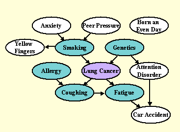
LUCAS

Competition rules

  • Conditions of participation: Anybody who complies with the rules of the challenge is welcome to participate. The challenge is part of the competition program of the World Congress on Computational Intelligence (WCCI08), Hong-Kong June 1-6, 2008. Participants are not required to attend the post-challenge workshop, which will be held at the conference, and the workshop is open to non-challenge participants. The proceedings of the competition will be published by the Journal of Machine Learning Research (JMLR).
  • Anonymity: All entrants must identify themselves with a valid email address, which will be used for the sole purpose of communicating with them. Emails will not appear on the result page. Name aliases are permitted during the development period to preserve anonymity. For all final submissions, the entrants must identify themselves by their real names.
  • Data: There are 4 datasets available (REGED, SIDO, CINA and MARTI), which have been progressively introduced, see the Dataset page. No new datasets will be introduced until the end of the challenge.
  • Development period: Results must be submitted beween the start and the termination of the challenge (the development period). The challenge starts on December 15, 2007 and is scheduled to terminate on April 30, 2008.
  • Submission method: The method of submission is via the form on the Submission page. To be ranked, submissions must comply with the Instructions. A submission may include results on one or several datasets. Please limit yourself to 5 submissions per day maximum. If you encounter problems with the submission process, please contact the Challenge Webmaster.
  • Ranking: For each entrant, only the last valid entry, as defined in the Instructions will count towards determining the winner. Valid entries are found in the Overall table. The method of scoring is posted on the Evaluation page. If the scoring method changes, the participants will be notified by email by the organizers.
  • Reproducibility: Everything is allowed that is not explicitly forbidden. We forbid using the test set for “learning from unlabeled data” [why?], that is for determining the structure and parameters of the model, including but not limited to learning variable causal dependencies from the test data, learning distribution shifts, and transduction. Participation is not conditioned on delivering your code nor publishing your methods. However, we will ask the top ranking participants to voluntarily cooperate to reproduce their results. This will include filling out a fact sheet about their methods and eventually participating to post-challenge tests and sending us their code, including the source code. The outcome of our attempt to reproduce your results will be published and add credibility to your results.

Challenge Datasets

We propose datasets from various application domains. We took great care of using real data. Some datasets encode real data directly, while others result from “re-simulation”, i.e. they were obtained from data simulators trained on real data. All datasets differing in name only by the last digit have the same training set. Digit zero indicates unmanipulated test sets. See the details of our data generating process.


Dataset (click for info) Description Test data Variables (num) Target Training examples Test examples Download (text format) Download (Matlab format)
REGED0 Genomics re-simulated data Not manipulated Numeric (999) Binary 500 20000 31 MB 25 MB
REGED1 Genomics re-simulated data Manipulated (see list of manipulated variables) Numeric (999) Binary 500 20000 31 MB 25 MB
REGED2 Genomics re-simulated data Manipulated Numeric (999) Binary 500 20000 31 MB 25 MB
SIDO0 Pharmacology real data w. probes Not manipulated Binary (4932) Binary 12678 10000 12 MB 14 MB
SIDO1 Pharmacology real data w. probes Manipulated Binary (4932) Binary 12678 10000 12 MB 14 MB
SIDO2 Pharmacology real data w. probes Manipulated Binary (4932) Binary 12678 10000 12 MB 14 MB
CINA0 Census real data w. probes Not manipulated Mixed (132) Binary 16033 10000 1 MB 1 MB
CINA1 Census real data w. probes Manipulated Mixed (132) Binary 16033 10000 1 MB 1 MB
CINA2 Census real data w. probes Manipulated Mixed (132) Binary 16033 10000 1 MB 1 MB
MARTI0 Genomics re-simulated data w. noise Not manipulated Numeric (1024) Binary 500 20000 47 MB 35 MB
MARTI1 Genomics re-simulated data w. noise Manipulated Numeric (1024) Binary 500 20000 47 MB 35 MB
MARTI2 Genomics re-simulated data w. noise Manipulated Numeric (1024) Binary 500 20000 47 MB 35 MB


A small example

We provide a small toy example dataset for practice purpose. You may submit results on these data on the Submit page like you would do for the challenge datasets. Your results will appear on the Result page, thus providing you with immediate feed-back. The results on these practice datasets WILL NOT COUNT as part of the challenge.
You may download all the example data as a single archive (Text format 1.1 MB, Matlab format 1.2 MB), or as individual datasets from the table below.


Dataset (click for info) Description Test data Variables (num) Target Training examples Test examples Download (text format) Download (Matlab format)
LUCAS0 Toy medicine data Not manipulated Binary (11) Binary 2000 10000 31 KB 22 KB
LUCAS1 Toy medicine data Manipulated Binary (11) Binary 2000 10000 31 KB 22 KB
LUCAS2 Toy medicine data Manipulated Binary (11) Binary 2000 10000 31 KB 22 KB
LUCAP0 Toy medicine data w. probes Not manipulated Binary (143) Binary 2000 10000 341 KB 262 KB
LUCAP1 Toy medicine data w. probes Manipulated Binary (143) Binary 2000 10000 342 KB 654 KB
LUCAP2 Toy medicine data w. probes Manipulated Binary (143) Binary 2000 10000 342 KB 263 KB


Dataset Formats

All datasets are formatted in a similar way. They include a training set from a “natural” distribution, in the form of a data table with variables in columns and samples in the rows. One particular column called “target” is singled out. A larger test set in the same format is provided, without the targets. The test set is not necessarily drawn from the same distribution as the training set. In particular, some variables may have been “manipulated”, i.e. an external agent may have set them to given values, therefore de facto disconnecting them from their natural causes.All data sets are in the same format and include 4 files in text format:

  • dataname.param – Parameters and statistics about the data.
  • dataname_train.data – Training set (a space delimited table with patterns in rows, features in columns).
  • dataname_test.data – Test set (same format as training set).
  • dataname_train.targets – Target velues for training examples.

For convenience, we also provide the data tables in Matlab format: dataname_train.mat and dataname_test.mat.

If you are a Matlab user, you can download some sample code to read and check the data.

How to format and ship results

Results File Formats

The results on each dataset should be formatted in text files according to the following table. If you are a Matlab user, you may find some of the sample code routines useful for formatting the data. You can view an example of each format from the filename column.


Filename Development Final entries Description File Format
[dataname]_feat.ulist Optional Compulsory (unless [dataname]_feat.slist is given) Unsorted list of N features used to make predictions. A space-delimited unsorted list of variables/features used to make prediction of the target variable. The features are numbered starting from 1, in the column order of the data tables.
[dataname]_feat.slist Optional Compulsory (unless [dataname]_feat.ulist is given) Sorted list of N features used to make predictions. A space-delimited sorted list of variables/features, most likely to be predictive come first. The features are numbered starting from 1, in the column order of the data tables. The list should contain no repetition, but it may contain a subset of all features. As explained below, the list may be used to define nested subsets of n predictive features.
[dataname]_train.predict Optional Compulsory Target prediction result table for training examples. Target prediction values* for all M samples of the data tables. There are two possible formats: (1) a single column of M prediction values, obtained with all the features of [dataname]_feat.ulist or [dataname]_feat.slist, or (2) a space delimited table of predictions for a varying number of predictive features, with M lines and C columns. The second format may be used only in conjunction with a valid [dataname]_feat.slist file. Each column should represent the prediction values obtained with only the first n features of [dataname]_feat.slist, where n varies by powers of 2: 1, 2, 4, 8, … If the total number of features N in [dataname]_feat.slist is not a power of 2, the last column should correspond to using all N features. Hence C=log2(N)+1 or log2(N)+2.
[dataname]_test.predict Compulsory Compulsory Target prediction result table for test examples.

* If the targets are binary {+1, -1} values (two-class classification) the prediction values may either be binary {+1, -1} or discriminant positive or negative values (zero will be interpreted as a small positive value).

When you submit your results you get immediate feed-back on the Result page: a color code indicates in which quartile your performance lies. Explanations about the scoring measures are found on the Evaluation page.
IMPORTANT: To see your results in the “Overall” Result table, you must enter results for all the tasks whose data names differ only by the number in the same submission, e.g. for REGED, you must enter results for REGED0, REGED1, and REGED2. Only the entries figuring in that table will be considered for the final ranking and the challenge prizes.

Results Archive Format

Submitted files must be in either a .zip or .tar.gz archive format. You can download the example zip archive to help familiarise yourself with the archive structures and contents (the results were generated with the sample code). Submitted files must use exactly the same filenames as in the example archive. If you use tar.gz archives please do not include any leading directory names for the files. Use

zip results.zip *.predict *.slist [or *.ulist]

or

tar cvf results.tar *.predict *.slist [or *.ulist]; gzip results.tar

to create valid archives.

Evaluation

The main objective of the challenge is to make good predictions of the target variable. The datasets were designed such that the knowledge of causal relationships should help making better predictions in manipulated test sets. Hence, causal discovery is assessed indirectly via the test set performances or Tscore, which we will use for determining the winner. We also provide for information Fnum, Fscore, and Dscore, but will not use them for ranking participants. The scores found in the table of Results are defined as follows:

  • Causal Discovery:
    • Fnum: The number of features in [dataname]_feat.ulist or the best number of features used to make predictions with [dataname]_feat.slist.
    • Fscore: Score for the list of features provided (see details below). For sorted lists [dataname]_feat.slist, the most predictive features should come first to get a high score. For unsorted lists [dataname]_feat.ulist, the features provided should be highly predictive to get a high score.
  • Target Prediction:
    • Dscore: Discovery score evaluating the target prediction values [dataname]_train.predict.
    • Tscore: Test score evaluating the target prediction values [dataname]_test.predict.

    Presently, for the datasets proposed, the Tscore and Dscore are the training and test AUC (which are identical to the BAC in the case of binary predictions).

During the development period, the scores are replaced by xxxx, except for the toy datasets, which do not count for the competition. A color coding indicates in which quartile your scores lie. The actual results will be made visible only after the end of the challenge.

Performance Measure Definitions

The results of classification, obtained by thresholding the prediction values made by a discriminant classifier, may be represented in a confusion matrix, where tp (true positive), fn (false negative), tn (true negative) and fp (false positive) represent the number of examples falling into each possible outcome:


Prediction
Class +1 Class -1
Truth Class +1 tp fn
Class -1 fp tn

We define the sensitivity (also called true positive rate or hit rate) and the specificity (true negative rate) as:
Sensitivity = tp/pos
Specificity = tn/neg
where pos=tp+fn is the total number of positive examples and neg=tn+fp the total number of negative examples.

Balanced ACccuracy (BAC) and Balanced Error Rate (BER)

The balanced accuracy is the average of the sensitivity and the specificity, obtained by thresholding the prediction values at zero:
BAC = 0.5*(tp/(tp+fn) + tn/(tn+fp)).
The balanced error rate is its complement to one: BER = (1-BAC)

Area Under Curve (AUC)

The area under curve or AUC is defined as the area under the ROC curve. This area is equivalent to the area under the curve obtained by plotting sensitivity against specificity by varying a threshold on the prediction values to determine the classification result. The AUC is calculated using the trapezoid method. In the case when binary scores are supplied for the classification instead of discriminant values, the curve is given by {(0,1),(tn/(tn+fp),tp/(tp+fn)),(1,0)} and AUC = BAC.
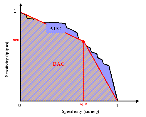
ROC

Fscore

To provide a more direct evaluation of causal discovery, we compute various scores, which evaluate the fraction of causes, effects, spouses, and other features, which may be related to the target, in the feature set that you are using to make predictions. We will use those scores to analyze the results of the challenge. One of those, which we call Fscore, is displayed in the Result tables. The Fscore is computed in the following way:

  • A set of “good” features is defined from the truth values of the causal relationships, known only to the organizers. This constitutes the “positive class” of the features. The other features belong to the “negative class”.
  • The features returned by the participants as a ulist or an slist are interpreted as classification results into the positive or negative class. For a ulist, all the list elements are interpreted as classified in the positive class and all other features as classified in the negative class. For an slist, the feature rank is mapped to a classification prediction value, the features ranking first being mapped to a high figure of merit. If the slist does not include all features, the missing features are all given the same lowest figure of merit.
  • The Fscore is the AUC for the separation “good” vs. “not-so-good” features. It is identical to the BAC in the case of a ulist.
  • The definition of “good” feature depends on the dataset and whether the test data are manipulated of not.
    • For artificial and re-simulated data (for which we know the all truth values of the causal relationships), the Test data Markov Blanket (MBT) is our chosen set of “good” features. The MBT generally does NOT coincides with the Discovery data Markov Blanket (MBD) of the natural distribution, from which discovery/training data are drawn, except if the test data were drawn from the same “unmanipulated” distribution.
    • For real data with probes (for which we know only the truth values of the causal relationships between target and probes), the set of “not-so-good” features is the set of probes not belonging to the Markov blanket of the target, in test data. In the case of manipulated data, since we manipulate all the probes, the set of “not-so-good” features coincides with the set of all probes. In this last case, if we define Rscore (“real score”) as the score for the separation of real variable into “cause” vs. “non-cause”, under some conditions, the Fscore is asymptotically linearly related to the Rscore

      Fscore = (num_true_pos/num_R) Rscore + 0.5 (num_true_neg/num_R)

      where num_true_pos is the (unknown) number of features in the true positive class (real variables, which are causes of the target) and, num_true_neg is the umber of other real variables, and num_R is the total number of real variables.


Listeners outperform automatic speech recognition systems at every level, including the very basic level of consonant identification. What is not clear is where the human advantage originates. Does the fault lie in the acoustic representations of speech or in the recognizer architecture, or in a lack of compatibility between the two? Many insights can be gained by carrying out a detailed human-machine comparison. The purpose of the Interspeech 2008 Consonant Challenge is to promote focused comparisons on a task involving intervocalic consonant identification in noise, with all participants using the same training and test data. This paper describes the Challenge, listener results and baseline ASR performance. Index Terms: consonant perception, VCV, humanmachine performance comparisons.

In most comparisons of human and machine performance on speech tasks, listeners win [1][2][3] (but see [4]; for an overview, see0[5]). While some of the benefit comes from the use of high-level linguistic information and world knowledge, listeners are also capable of better performance on low-level tasks such as consonant identification which do not benefit from lexical, syntactic, semantic and pragmatic knowledge. This is especially the case when noise is present. For this reason, understanding consonant perception in quiet and noisy conditions is an important scientific goal with immediate applications in speech perception (e.g. for the design of hearing prostheses) and spoken language processing [6]. A detailed examination of confusion patterns made by humans and computers can point towards potential problems at the level of speech signal representations or recognition architectures. For example, one compelling finding from a number of recent studies has been that much of the benefit enjoyed by listeners comes from better perception of voicing distinctions [7][8][9]. A number of corpora suitable for speech perception testing exist [7][10], although few contain sufficient data to allow training of automatic speech recognizers. However, the main motivation for the Interspeech 2008 Consonant Challenge was not solely to make available a corpus large enough for human-machine comparisons, but also to define a number of varied and challenging test conditions designed to exercise listeners and algorithmic approaches. In addition, by providing software for perceptual testing and scoring, the aim was to support a wide range of comparisons, for both native and non-native listeners. This paper describes the design, collection and postprocessing of the Consonant Challenge corpus and specifies the test conditions as well as the training and development material. It provides results for native listeners and for two baseline automatic speech recognition systems.

The Challenge

Listeners outperform automatic speech recognition systems at every level of speech recognition, including the very basic level of consonant recognition. What is not clear is where the human advantage originates. Does the fault lie in the acoustic representations of speech or in the recogniser architecture, or in a lack of compatibility between the two? There have been relatively few studies comparing human and automatic speech recognition on the same task, and, of these, overall identification performance is the dominant metric. However, there are many insights which might be gained by carrying out a far more detailed comparison.

The purpose of this Special Session is to promote focused human-computer comparisons on a task involving consonant identification in noise, with all participants using the same training and test data. Training and test data and native listener and baseline recogniser results will be provided by the organisers, but participants are encouraged to also contribute listener responses.

Contributions are sought in (but not limited to) the following areas:

  • Psychological models of human consonant recognition
  • Comparisons of front-end ASR representations
  • Comparisons of back-end recognisers
  • Exemplar vs statistical recognition strategies
  • Native/Non-native listener/model comparisons

The results of the Challenge will be presented at a Special Session of Interspeech’08 in Brisbane, Australia.

Speakers and VCV material

Twelve female and 12 male native English talkers aged between 18-49 contributed to the corpus. Speakers produced each of the 24 consonants (/b/, /d/, /g/, /p/, /t/, /k/, /s/, //, /f/, /v/, //, //, /t/, /z/, //, /h/, /d/, /m/, /n/, //, /w/, //, /y/, /l/) in nine vowel contexts consisting of all possible combinations of the three vowels /i:/ (as in “beat”), /u:/ (as in “boot”), and /ae/ (as in “bat”). Each VCV was produced using both front and back stress (e.g. ‘aba vs ab’a) giving a total of 24 (speakers) * 24 (consonants) * 2 (stress types) * 9 (vowel contexts) = 10368 tokens. Pilot listening tests were carried out to identify unusable tokens due to poor pronunciations or other problems.
See the Technical details page for further details of the collection and postprocessing procedure.

Training, development and test sets

Training material comes from 8 male and 8 female speakers while tokens from the remaining 8 speakers are used in the independent test set. A development set will be released shortly. After removing unusable tokens identified during post-processing, the training set consists of 6664 clean tokens.

Seven tests sets, corresponding to a quiet and 6 noise conditions, are available. Each test set contains 16 instances of each of the 24 consonants, for a total of 384 tokens. Listeners will identify consonants in each of the test conditions. Minimally, each contribution to the special session should report results on some or all of the test sets. Scoring software will be released in February 2008.

Noise

The table shows the 7 conditions:


test set noise type SNR (dB)
1 clean
2 competing talker -6
3 8-talker babble -2
4 speech-shaped noise -6
5 factory noise 0
6 modulated speech-shaped noise -6
7 3-speaker babble -3

These noise types provide a challenging and varied range of conditions. Signal-to-noise ratios were determined using pilot tests with listeners with the goal of producing similar identification scores (~ 65-70%) in each noise condition.

VCV tokens are additively embedded in noise samples of duration 1.2s. The SNR is computed token-wise and refers to the SNR in the section where the speech and noise overlap. The time of onset of each VCV takes on one of 8 values ranging from 0 to 400 ms.

In addition, test materials are also available as “stereo” sound files which are identical to the test sets except that the the noise and VCV tokens are in separate channels. We have made the test material available in this form to support computational models of human consonant perception which may wish to make some assumptions about e.g. ideal noise processing, and also to allow for the computation of idealised engineering systems (e.g. to determine performance ceilings). Of course, contributors should clearly distinguish which of their results are based on the single-channel and dual-channel noise sets.

Download training, test, and development material.

Experimental Set-up

Twenty seven native English listeners aged between 18 and 48 who reported no hearing problems identified the 384 VCVs of the test set. Listeners were drawn from the staff and students at the University of Sheffield and were paid for their participation. Perception tests ran under computer control in the IAC booth. Listeners were presented with a screen layout as shown in Figure 1 on which the 24 consonants were represented using both ASCII symbols and with an example word containing the sound. Listeners were phonetically-naive and were given instructions as to the meaning of each symbol. They underwent a short practice session prior to the main test. Two listeners failed to reach a criterion level of 85% in a practice session using clean tokens. Another failed to complete all conditions, while a fourth was an outlier on most of the test conditions. Results are reported for the remaining 23 listeners. For the main test, listeners started with the clean condition. The order of the noisy conditions was randomised.

We welcome further contributions of listener results from native British English, other native English and non-native populations. We can make available MATLAB software for running listening tests if needed. Note that we anticipate that listening to the full range of tests will take 90-120 minutes in addition to the time taken for hearing tests and practice. Please contact the organisers for further information and to ensure that potential contributions are as useful as possible.

Results

The native listener results, averaged over all consonants and all listeners, are shown in the table below for each of the test conditions separately:

Test set 1 2 3 4 5 6 7
Rec. rate 93.8 79.5 76.5 72.2 66.7 79.2 71.4
Std. err. 0.57 0.78 0.79 0.75 0.77 0.61 0.74

Confusions matrices and Transmitted Information has been calculated for each of the test conditions separately:

The diagonal of the confusion matrices shows the percentage correct responses. Vertically: the phoneme that was produced; horizontally: the phoneme that was recognised.

The table used to calculate the Transmitted Information for manner, place, and voicing can be downloaded here.

The baseline recognition system

The performance of various acoustic features (MFCC, FBANK, MELSPEC, Ratemaps) and recogniser architectures (monophone, triphone, gender-dependent/independent) was investigated. Two representative combinations were chosen as baselines for the Consonant Challenge: one system based on MFCCs, the other on Ratemaps.

For both systems, 30 models were trained, 24 consonants and two models for each of the three vowels – one to model the initial vowel context and one to model the final vowel context of the VCV. The maximum number of training items per consonant is 9 (vowel contexts) * 2 (stress conditions) * 16 (speakers) = 288 items.

MFCC-based recognition system

The speech is parameterised with 12 MFCC coefficients and log energy and augmented with first and second temporal derivatives resulting in a 39-dimensional feature vector. Each of the monophones consists of 3 emitting states with a 24-Gaussian mixture output distribution. No silence model and short pause model are employed in this distribution as features are end-pointed. The HMMs were trained from a flat start using HTK.

Ratemap-based recognition system

Ratemaps are a filterbank-based representation based on auditory excitation patterns. 64-dimensional feature vectors and the same model architecture as for the MFCC-based system were used.

A .zip file containing the MFCC-based baseline model, training and testing scripts, and the evaluation script can be downloaded here. The ratemap generation scripts are available upon request. A short explanation of the scripts can be downloaded here. For any remaining questions please contact Ning Ma (University of Sheffield, UK).

Results

The overall consonant recognition accuracy for the MFCC-based recognition system is 88.5% on Test set 1 (clean). The overall consonant recognition accuracy for the Ratemap-based system on Test set 1 is 84.4%.

The confusion matrices of the two baseline systems can be found here. The diagonal of the confusion matrices shows the number of correct responses (16 is the maximum). Vertically: the phoneme that was produced; horizontally: the phoneme that was recognised.

The speech material

A description of the material can be found on the Description of the materials page.

The .zip files of both sets of test material and the development material contain seven directories, named testsetX and devsetX where X is the number referring to the number associated with the type of noise in the table on the Description of the materials page. In addition to this, test.zip also contains seven directories named testsetXp. These contain a small number of practice stimuli, which can be used in the perceptual experiments to give the listeners a small practice session. If you are not running perceptual experiments, you can ignore these directories. Finally, the test.zip and dev.zip also contain six files named testsetX_offsets.dat and devsetX_offsets.dat. These are (MATLAB) files showing the offsets of each of the VCVs into the noise. People building ASR systems are not allowed to use these data.

Phoneme segmentation data

The models of the MFCC-based baseline recognition system (click here for a description of the model set) were used to create phoneme segmentations of the clean test data using forced alignment.

Warning: Everyone is invited to use these segmentations but should be warned that they are not ‘perfect’ segmentations. If you obtain better segmentations and if you would like to share these please send them to the organisers via e-mail and we will post them on this website.

A number of people are helping us with the realisation of this Challenge. Many thanks go out to them!

  • The PASCAL Network: for financial support.
  • Maria Luisa Garcia Lecumberri (University of the Basque Country, Spain): for help with the design of the speech material, analysis of the production material, and the design of listening experiments.
  • Ning Ma (University of Sheffield, UK): for on-going work on the baseline recogniser.
  • Youyi Lu (University of Sheffield, UK): for helping run the listening experiments.
  • Matt Gibson (University of Sheffield, UK): for discussions on the baseline speech recogniser.

Stemmatology (a.k.a. stemmatics) studies relations among different variants of a document that have been gradually built from an original by copying and modifying earlier versions. The aim of such study is to reconstruct the family tree of the variants.

We invite applications of established and, in particular, novel approaches, including but of course not restricted to hierarchical clustering, graphical modeling, link analysis, phylogenetics, string-matching, etc.

The objective of the challenge is to evaluate the performance of various approaches. Several sets of variants for different texts are provided, and the participants should attempt to reconstruct the relationships of the variants in each data-set. This enables the comparison of methods usually applied in unsupervised scenarios.

Data

The data is available in plain text format. It is under consideration whether some more pre-processed formats will be made available in order to reduce the effort of the participants. In any case, the plain text versions will remain available, and can be used in the challenge — since pre-processing is likely to lose some information, some methods may benefit from using the original data.

There is one primary data-set which is used to determine the primary ranking of the participants. The total number of points earned in all of the data-sets (excluding the primary one) will be used as a secondary ranking scheme. For more information on the ranking schemes, see the Rules.


Disclaimer: All the data-sets are provided only for use related to the challenge. Further use of the data requires an explicit permission by the organizers and the original providers of the data.

About the Nexus format: The conversion from plain (aligned) text to the Nexus format was performed by ordering at each ‘locus’ (a place in the text) the words that appear in the locus in alphabetical order, and by assigning to each variant a symbol (A,B,C,…). Thus, if three different variants of a given word appear in the texts, then the symbols A,B, and C appear in the Nexus file at the same locus. Missing words are replaced by a question mark (?). The Nexus files are directly compatible with, for instance, the PAUP* software. (See the Results.)

Primary Data-Set: Heinrichi

The primary data-set is a result of an experiment performed by the organizers and 17 volunteers (see Credits). The original text is in old Finnish, and is known as Piispa Henrikin surmavirsi (‘The Death-Psalm of Bishop Henry’).

Some of the copied variants are ‘missing’, i.e., not included in the given data-set. The copies were made by hand (pencil and paper). Note that the structure of the possible stemma is not necessarily limited to a bifurcating tree: more than two immediate descendants (children) and more than one immediate predecessor (parents) are possible.

New: The correct stemma and an evaluation script are available at the Causality workbench.

Data-Set #2: Parzival (Validation Data)

This is also an artificial data-set made by copying a text by hand. The correct solution will be made available during the challenge in order to enable self-assessment. This data-set will not affect the final results.

'' If vaccilation dwell with the heart, the soul will see it. 
Shame and honour clash with the courage of a steadfast man is motley like a magpie. 
But such a man may yet make merry, for Heaven & Hell have equal part in him. ... ''

The text is the beginning of the German poem Parzival by Wolfram von Eschenbach, translated to English by A.T. Hatto. The data was kindly provided to us by Matthew Spencer and Heather F. Windram.

Data-Set #3: Notre Besoin

Another artificial data-set. The text is from Stig Dagerman’s, Notre besoin de consolation est impossible à rassasier, Paris: Actes Sud, 1952 (translated to French from Swedish by P. Bouquet), kindly provided to us by Caroline Macé.

'' Je suis dépourvu de foi et ne puis donc être heureux, car un homme qui risque
de craindre que sa vie ne soit errance absurde vers une mort certaine ne peut
être heureux. ... ''

Data-Set #4: Legend of St. Henry

This is a real data-set. The text is the Legend of St. Henry of Finland in Latin, written by the end of the 13th century at the latest. The surviving 52 versions are provided, some of which are severely damaged and fragmentary.

For ease of use, the texts are aligned so that each line in the file contains one word, and empty lines are added so that the lines match across different files (e.g. the 50th line in each file contains the word pontificem unless that part of the manuscript is missing or damaged). The text is roughly 900 words long.

Procedures

There are several data-sets included in the challenge. Some of them are real transcribed medieval manuscripts, some artificial (but hand-copied) ones. The data-sets are made available in (at least) two phases. Correct answers to some of the first phase data-sets will be announced before the final submission deadline in order to enable self-assessment by the participants. These data-sets will not affect the final results.

Submissions are made in groups (of size one or more persons). Each group should submit at most two solutions. If more than two solutions are submitted, the last two before the deadline are accepted. A person can belong to at most two groups. (So a person can contribute to a maximum of four solutions.)

Evaluation

For the artificial data-sets, for which there is a known ‘ground-truth’ solution, the difference between the proposed and correct solutions is evaluation. The exact criterion is open for discussion among participants (and other interested parties). The current scoring function is based on distance orders among triplets (for details, see Example)  Go to Discussion.

For the real data-sets, there is no known correct solution. Therefore, EBS¹ will be used: the ‘owner’ of the data-set will be asked to estimate whether the proposed solution is plausible and useful from his/her point of view.


¹ EBS: endorphin-based scoring

Ranking Schemes

There are two ranking schemes.

  • Primary ranking is based on performance on the primary data-set (see Data Sets).
  • Secondary ranking is based on all the other data sets except those for which the correct solution is annouced during the challenge, including both artificial and real data. For these other data sets, ‘thumbs-up’ marks will be awarded to the best submissions, and the total number of thumbs up determines the secondary ranking.

The organizers reserve the right to alter the rules of the challenge at any point.

Restrictions

Anyone who has been in contact with some of the data-sets, or has otherwise obtained inside information about the correct solution should obviously not enter the challenge as regards the data-set(s) in question. However, participation is allowed as regards the other data-sets.

The data-sets are provided only for the use in the challenge. Further use of the data requires an explicit permission by the organizers and the original providers of the data.

Results

Team*   Method** Data #1 Data #2 Data #3 Data #4***
Team Demokritos  n-gram clustering 64.4 % 79.3 % 66.4 %
Rudi Cilibrasi CompLearn 52.7 % 81.5 % 70.6 %
Hierarchical clustering 72.6 % 60.2 %
 RHM06 76.0 % 79.9 % 76.9 %
 PAUP: Parsimony 74.4 % 77.8 % 74.5 %
 PAUP: Neighbour Joining 64.4 % 81.5 % 76.2 %
 PAUP: Least Squares 64.2 % 81.5 % 70.2 %
 SplitsTree: NeighborNet 59.1 % 77.8 % 70.2 %
 SplitsTree: SplitDecomposition 53.1 % 74.5 % 73.1 %
 SplitsTree: ParsimonySplits 56.8 % 83.7 % 71.6 %

*) The entries below the horizontal line are added for comparison purposes by the organizers, and, therefore, not included in the competition.

**) RHM06 = (Roos, Heikkilä, Myllymäki, “A Compression-Based Method for Stemmatic Analysis”, ECAI-06).
PAUP = PAUP* version 4.0b10 for Unix. Heuristic search.
SplitsTree = SplitsTree4 version 4.10, build 2, May 2008.

***) Data #4 is ‘real’ and no correct solution is known.

The winner in the primary ranking (Data #1) is Team Demokritos (click on the team title in the table for more information).

The secondary ranking is based on Data #3 and Data #4 for which the winner is Rudi Cilibrasi who’s submission was the best for Data #3. Neither submission was “plausible and useful” for Data #4 (as judged by a domain expert, hence no points for anyone).


The objective of the Challenge is to design a statistical machine learning algorithm that discovers which morphemes (smallest individually meaningful units of language) words consist of. Ideally, these are basic vocabulary units suitable for different tasks, such as text understanding, machine translation, information retrieval, and statistical language modeling.

The scientific goals are:

  • To learn of the phenomena underlying word construction in natural languages
  • To discover approaches suitable for a wide range of languages
  • To advance machine learning methodology

Morpho Challenge 2007 is a follow-up to our previous Morpho Challenge 2005 (Unsupervised Segmentation of Words into Morphemes). The task of Morpho Challenge 2007 is more general in that we are not necessarily looking for an explicit segmentation of words this time, but a morpheme analysis of the word forms in the data. (For instance, the English words “boot, boots, foot, feet” might obtain the analyses “boot, boot + plural, foot, foot + plural”, respectively.)

Participation in the previous challenge is by no means a prerequisite for participation in Morpho Challenge 2007. Everyone is welcome and we hope to attract many participating teams. The results will be presented in a workshop arranged in conjunction with CLEF 2007 (Cross-Language Evaluation Forum). Please read the rules and see the schedule. The datasets are available for download. Submit your analyses (result files) by sending them by email to the organizers, or by indicating a location where the organizers can download your files. Remember also to describe your algorithm in an extended abstract. Please read the formatting instructions in rules.

The result tables from the latest evaluation runs are now in the Results page.

We are looking forward to an interesting competition!

Mikko Kurimo, Mathias Creutz and Matti Varjokallio
Adaptive Informatics Research Centre, Helsinki University of Technology
The organizers

Program committee

Levent Arslan, Boğaziçi University
Eric Atwell, University of Leeds
Samy Bengio, Google
Tolga Cilogu, Middle-East Technical University
Kadri Hacioglu, Colorado University
Colin de la Higuera, Jean Monnet University, Saint-Etienne
Chun Yu Kit, City University of Hong Kong
Dietrich Klakow, Saarland University
James Martin, University of Colorado at Boulder
Jan Nouza,Technical University of Liberec
Erkki Oja, Helsinki University of Technology
Murat Saraçlar, Boğaziçi University
Richard Sproat, University of Illinois, Urbana-Champaign
Richard Wicentowski, Swarthmore College

Rules

Acceptance

The organizers retain all rights to the Challenge data, which is given to the participants for use in this challenge only. The organizers may use the data submitted to the Challenge freely, without restrictions.

Eligibility

Anyone is allowed to participate. A participant may be either a single person or a group. A single person can participate in at most two groups. A participant is allowed to submit at most three different solutions, where each solution corresponds to a particular morpheme analysis method. Each of these methods may naturally be applied to each of the test languages. If a participant submits more than three solutions, the organizers decide which of the three will be accepted.

Test languages

Data sets are provided for four languages: English, Finnish, German and Turkish. Participants are encouraged to apply their algorithm to all of these test languages, but are free to leave some languages out, if they wish to do so.

(New languages may be added, if interested co-organizers, suitable data and evaluation analyses become available in time.)

Task

The task is the unsupervised morpheme analysis of every word form contained in a word list supplied by the organizers for each test language.

The participants will be pointed to corpora in which the words occur, so that the algorithms may utilize information about word context.

Solutions, in which a large number of parameters must be “tweaked” separately for each test language, are of little interest. This challenge aims at the unsupervised (or very minimally supervised) morpheme analysis of words. The abstracts submitted by the participants must contain clear descriptions of which steps of supervision or parameter optimization are involved in the algorithms.

Competitions

The segmentations will be evaluated in two complementary ways:

  • Competition 1: The proposed morpheme analyses will be compared to a linguistic “gold standard”.
  • Competition 2: Information retrieval (IR) experiments will be performed, where the words in the documents and queries will be replaced by their proposed morpheme representations. The search will then be based on morphemes instead of words.

Competition 1 will include all four test languages. Winners will be selected separately for each language. As a performance measure, the F-measure of accuracy of suggested morpheme analyses is utilized. Should two solutions produce the same F-measure, the one with higher precision will win.

Competition 2 will include three of the test languages. The organizers will perform the IR experiments based on the morpheme analyses submitted by the participants.

Workshop and publication

All good results will be acknowledged with fame and glory. Presentations for the challenge workshop will be selected by the program committee based on the results and an extended abstract of at most 6 pages.

Extended abtracts

For the extended abstract you can use the two-column ACL/COLING format (figures and tables may still span the whole width of a page). Detailed formatting instructions can be found here: PDF or PS. You can use the following files: Latex style file, Latex bibliography file, and a template Latex document. The maximum length of your paper is 6 pages (including references and figures). Email your extended abstract to the organizers by May 31.

Camera-ready submission

The final camera-ready submissions use a different format than the papers submitted for review. We are sorry about the inconvenience of your having to reformat your documents. For your final paper submission (due August 15th), please use the single-column CLEF 2007 Notebook Proceedings format. Here are a sample PDF file and a template Latex document. Detailed formatting instructions can be requested from the Morpho Challenge Organizers. The maximum length of your paper is 10 pages (including references and figures), but you can ask for a couple of extra pages if you think it improves the paper. Email your final paper to the organizers.

Arbitration

In the case of disagreement the organizers will decide the final interpretation of the rules.

Datasets

There are a number of data files involved in this challenge. Each type of file is available for each language.

Word list (input)

First and foremost, there is a list of word forms. The words have been extracted from a text corpus, and each word in the list is preceded by its frequency in the corpus used.

For instance, a subset of the supplied English word list looks like this:

...
1 barefoot's
2 barefooted
6699 feet
653 flies
2939 flying
1782 foot
64 footprints
...

Result file (output, i.e., what to submit)

The participants’ task is to return a list containing exactly the same words as in the input, with morpheme analyses provided for each word. The list returned shall not contain the word frequency information.

A submission for the above English words may look like this:

...
barefoot's      BARE FOOT +GEN
barefooted      BARE FOOT +PAST
feet            FOOT +PL
flies           FLY_N +PL, FLY_V +3SG
flying          FLY_V +PCP1
foot            FOOT
footprints      FOOT PRINT +PL
...

There are a number of things to note about the result file: Each line of the file contains a word (e.g., “feet”) separated from its analysis (e.g., “FOOT +PL”) by one TAB character. The word needs to look exactly as it does in the input; no capitalization or change of character encoding is allowed. The analysis contains morpheme labels separated using space. The order in which the labels appear does not matter; e.g., “FOOT +PL” is equivalent to “+PL FOOT”. The labels are arbitrary: e.g., instead of using “FOOT” you might use “morpheme784” and instead of “+PL” you might use “morpheme2”. However, we strongly recommend you to use intuitive labels, when possible, since they make it easier for anyone to get an idea of the quality of the result by looking at it.

If a word has several interpretations, all interpretations should be supplied: e.g., the word “flies” may be the plural form of the noun “fly” (insect) or the third person singular present tense form of the verb “to fly”. The alternative analyses must be separated using a comma, as in: “FLY_N +PL, FLY_V +3SG”. The existence of alternative analyses makes the task challenging, and we leave it to the participants to decide how much effort they will put into this aspect of the task. In English, for instance, in order to get a perfect score, it would be necessary to distinguish the different functions of the ending “-s” (plural or person ending) as well as the different parts-of-speech of the stem “fly” (noun or verb). As the results will be evaluated against reference analyses (our so-called gold standard), it is worth reading about the guiding principles used when constructing the gold standard.

As far as we understand, you can use any characters in your morpheme labels except whitespace and comma (,). However, we cannot guarantee that the evaluation scripts will work properly, if your labels contain some “strange” characters.

Text corpus

The word list (input data) has been constructed by collecting word forms occurring in a text corpus. The text corpora have been obtained from the Wortschatz collection at the University of Leipzig (Germany). We used the plain text files (sentences.txt for each language); the corpus sizes are 3 million sentences for English, Finnish and German, and 1 million sentences for Turkish. For English, Finnish and Turkish we use preliminary corpora, which have not yet been released publicly at the Wortschatz site. The corpora have been preprocessed for the Morpho Challenge (tokenized, lower-cased, some conversion of character encodings).

If the participants like to do so, they can use the corpora in order to get information about the context in which the different words occur.

We are most grateful to the University of Leipzig for making these resources available to the Challenge, and in particular we thank Stefan Bordag for his kind assistance.

Gold standard morpheme analyses

The desired “correct” analyses for a random sample of circa 500 words are supplied for each language. These samples can be used for visual inspection and as a development test set (in order to get a rough estimate of the performance of the participants’ morpheme-analyzing algorithm).

The format of the gold standard file is exactly the same as that of the result file to be submitted. That is, each line contains a word and its analysis. The word is separated from the analysis by a TAB character. Morpheme labels in the analysis are separated from each other by a space character. For some words there are multiple correct analyses. These alternative analyses are separated by a comma (,). Examples:

Language Examples
English baby-sitters       baby_N sit_V er_s +PL
indoctrinated      in_p doctrine_N ate_s +PAST
Finnish linuxiin           linux_N +ILL
makaronia          makaroni_N +PTV
German choreographische   choreographie_N isch +ADJ-e
zurueckzubehalten  zurueck_B zu be halt_V +INF
Turkish kontrole           kontrol +DAT
popUlerliGini      popUler +DER_lHg +POS2S +ACC, popUler +DER_lHg +POS3 +ACC3

The English and German gold standards are based on the CELEX data base. The Finnish gold standard is based on the two-level morphology analyzer FINTWOL from Lingsoft, Inc. The Turkish gold-standard analyses have been obtained from a morphological parser developed at Boğaziçi University; it is based on Oflazer’s finite-state machines, with a number of changes. We are indebted to Ebru Arısoy for making the Turkish gold standard available to us.

The morphological analyses are morpheme analyses. This means that only grammatical categories that are realized as morphemes are included. For instance, for none of the languages will you find a singular morpheme for nouns or a present-tense morpheme for verbs, because these grammatical categories do not alter or add anything to the word form, in contrast to, e.g., the plural form of a noun (house vs. house+s), or the past tense of verbs (help vs. help+ed, come vs. came).

The morpheme labels that correspond to inflectional (and sometimes also derivational) affixes have been marked with an initial plus sign (e.g., +PL, +PAST). This is due to a feature of the evaluation script: in addition to the overall performance statistics, evaluation measures are also computed separately for the labels starting with a plus sign and those without an initial plus sign. It is thus possible to make an approximate assessment of how accurately affixes are analyzed vs. non-affixes (mostly stems). If you use the same naming convention when labeling the morphemes proposed by your algorithm, this kind of statistics will be available for your output (see the evaluation page for more information).

The morpheme labels that have not been marked as affixes (no initial plus sign) are typically stems. These labels consist of an intuitive string, usually followed by an underscore character (_) and a part-of-speech tag, e.g., “baby_N”, “sit_V”. In many cases, especially in English, the same morpheme can function as different parts-of-speech; e.g., the English word “force” can be a noun or a verb. In the majority of these cases, however, if there is only a difference in syntax (and not in meaning), the morpheme has been labeled as either a noun or a verb, throughout. For instance, the “original” part-of-speech of “force” is a noun, and consequently both noun and verb inflections of “force” contain the morpheme “force_N”:

force force_N
force's force_N GEN
forced force_N +PAST
forces force_N +3SG, force_N +PL
forcing force_N +PCP1

Thus, there is not really a need for your algorithm to distinguish between different meanings or syntactic roles of the discovered stem morphemes. However, in some rare cases, if the meanings of the different parts-of-speech do differ clearly, there are two variants, e.g., “train_N” (vehicle), “train_V” (to teach), “fly_N” (insect), “fly_V” (to move through the air). But again, if there are ambiguous meanings within the same part-of-speech, these are not marked in any way, e.g., “fan_N” (device for producing a current of air) vs. “fan_N” (admirer). This notation is a consequence of using CELEX and FINTWOL as the sources for our gold standards. We could have removed the part-of-speech tags, but we decided to leave them there, since they carry useful information without significantly making the task more difficult. There are no part-of-speech tags in the Turkish gold standard.

Random word pairs file

If you want to carry out a small-scale evaluation yourself using the gold standard sample, you need to download a randomly generated so-called word pairs file for each language to be tested. Read more about this on the evaluation page.

Character encoding

In the source data used for the different languages, there is variation in how accurately certain distinctions are made when letters are rendered. This makes it hard to apply a unified character encoding scheme for all the languages (such as UTF-8). Thus, the following encodings have been used, in which all letters are encoded as one-byte (8-bit) characters:

English
Standard text. All words are lower-cased, also proper names.
Finnish
ISO Latin 1 (ISO 8859-1). The Scandinavian special letters å, ä, ö (as well as other letters occuring in loan words, e.g., ü, é, à) are rendered as one-byte characters. All words are lower-cased, also proper names.
German
Standard text. All words are lower-cased, also all nouns. The German umlaut letters are rendered as the corresponding non-umlaut letter followed by “e”, e.g., “laender” (Länder), “koennte” (könnte), “fuer” (für). Double-s is rendered as “ss”, e.g., “strasse” (Straße). This coarse encoding is due to the fact that CELEX, the source for the morphological gold standard, utilizes this scheme. Note, however, that in the data you may see special letters encoded using ISO Latin 1 in some loan words, e.g., “société”, “l’unità” (these words are not included in CELEX and their analyses will not be evaluated).
Turkish
Standard text. All words are lower-cased. The letters specific to the Turkish language are replaced by capital letters of the standard Latin alphabet, e.g., “açıkgörüşlülüğünü” is spelled “aCIkgOrUSlUlUGUnU”.

Download

Language Word list Text corpus Sample of gold standard Random word pairs file
English Text Text gzipped Text gzipped Text Text
Finnish Text Text gzipped Text gzipped Text Text
German Text Text gzipped Text gzipped Text Text
Turkish Text Text gzipped Text gzipped Text Text

Instead of downloading each file separately, you can download the whole package, either as a tar/gzip file: morphochal07data.tgz (530 MB; unpack using “tar xzf“) or as a zip file: morphochal07data.zip (540 MB).

Competition 1

In Competition 1, for each language, the morpheme analyses proposed by the participants’ algorithm will be compared against a linguistic gold standard. Samples of the gold standards used are available for download on the datasets page.

Since the task at hand involves unsupervised learning, it cannot be expected that the algorithm comes up with morpheme labels that exactly correspond to the ones designed by linguists. That is, no direct comparison will take place between labels as such (the labels in the proposed analyses vs. labels in the gold standard). What can be expected, however, is that two word forms that contain the same morpheme according to the participants’ algorithm also have a morpheme in common according to the gold standard. For instance, in the English gold standard, the words “foot” and “feet” both contain the morpheme “foot_N”. It is thus desirable that also the participants’ algorithm discovers a morpheme that occurs in both these word forms (be it called “FOOT”, “morpheme784”, “foot” or something else).

In practice, the evaluation will take place by sampling a large number of word pairs, such that both words in the pair have at least one morpheme in common. As the evaluation measure, we will use F-measure, which is the harmonic mean of Precision and Recall:

F-measure = 1/(1/Precision + 1/Recall).

Precision is here calculated as follows: A number of word forms will be randomly sampled from the result file provided by the participants; for each morpheme in these words, another word containing the same morpheme will be chosen from the result file by random (if such a word exists). We thus obtain a number of word pairs such that in each pair at least one morpheme is shared between the words in the pair. These pairs will be compared to the gold standard; a point is given for each word pair that really has a morpheme in common according to the gold standard. The total number of points is then divided by the total number of word pairs.

For instance, assume that the proposed analysis of the English word “abyss” is: “abys +s”. Two word pairs are formed: Say that “abyss” happens to share the morpheme “abys” with the word “abysses”; we thus obtain the word pair “abyss – abysses”. Also assume that “abyss” shares the morpheme “+s” with the word “mountains”; this produces the pair “abyss – mountains”. Now, according to the gold standard the correct analyses of these words are: “abyss_N”, “abyss_N +PL”, “mountain_N +PL”, respectively. The pair “abyss – abysses” is correct (common morpheme: “abyss_N”), but the pair “abyss – mountain” is incorrect (no morpheme in common). Precision here is thus 1/2 = 50%.

Recall is calculated analogously to recall: A number of word forms are randomly sampled from the gold standard file; for each morpheme in these words, another word containing the same morpheme will be chosen from the gold standard by random (if such a word exists). The word pairs are then compared to the analyses provided by the participants; a point is given for each sampled word pair that has a morpheme in common also in the analyses proposed by the participants’ algorithm. The total number of points is then divided by the total number of word pairs.

For words that have several alternative analyses, as well as for word pairs that have more than one morpheme in common, some normalization of the points is carried out in order not to give these words considerably more weight in the evaluation than “less complex” words. We will spare the participants from the gory details. (The passionately interested reader may have a look at the source code of the evaluation script.)

Evaluation of a sample (development test set)

You can evaluate your morphological analyses against the available gold standards (separately for each test language). The program to use for this is the Perl script: eval_morphemes.pl. The evaluation program is invoked as follows:

eval_morphemes.pl [-trace] wordpairsfile_goldstd wordpairsfile_result goldstdfile resultfile

Four files are given as arguments to eval_morphemes.pl:

  1. wordpairsfile_goldstd: this is the “random word pairs file” available for download on the datasets page. This file is needed in the calculation of an estimate of the recall of the proposed morpheme analyses.
  2. wordpairsfile_result: this file has to be generated using another program (see below). It is needed in the calculation of a rough estimate of the precision of the proposed morpheme analyses.
  3. goldstdfile:this is the sample of the gold standard available for download on the datasets page. This file contains the correct morpheme analyses for circa 500 words.
  4. resultfile: this is the result file that your algorithm produces, i.e., a list of words and their proposed morpheme analyses.

The -trace argument is optional and produces output for every evaluated word separately. Regardless of the status of the trace argument, the evaluation program produces output of the following kind:

PART0. Precision: 69.00% (96/139); non-affixes: 81.55% (51/63); affixes: 58.73% (45/76)
PART0. Recall:    25.59% (142/556); non-affixes: 49.78% (105/211); affixes: 10.78% (37/345)
PART0. F-measure: 37.33%; non-affixes: 61.82%; affixes: 18.22%
#
TOTAL. Precision: 69.00%; non-affixes: 81.55%; affixes: 58.73%
TOTAL. Recall:    25.59%; non-affixes: 49.78%; affixes: 10.78%
TOTAL. F-measure: 37.33%; non-affixes: 61.82%; affixes: 18.22%

Note that results are displayed for partition 0 (PART0) and for the entire data (TOTAL). The total scores are here the same as the scores of PART0, since there is only one partition. It is, however, possible to split the data into several partitions and compute results for each partition separately. The overall scores are then calculated as the mean over the partitions. Splitting into partitions is a feature reserved for the final evaluation, when we will assess the statistical significance of the differences between the participants’ algorithms.

The figures that count in the final evaluation are the first precision, recall, and F-measure values on the TOTAL lines. These values pertain to all morphemes, but there are also separate statistics for morphemes classified as non-affixes vs. affixes. What counts as an affix is a morpheme with a label starting with a plus sign, e.g., “+PL”, “+PAST”. This naming convention is applied in the gold standard, which means that you do not have to do anything in order to get the non-affixes/affixes statistics right as far as recall is concerned. However, if you want the same kind of information also for precision, your algorithm must have a means of discovering which morphemes are likely affixes and tag these morphemes with an initial plus sign. Note that it is fully up to you whether you do this or not; it will not affect your position in the competition in any way.

Sampling word pairs for the calculation of an estimate of the precision

In order to get an estimate of the precision of the algorithm, you need to provide the evaluation script eval_morphemes.pl with a file containing word pairs sampled from your result file. Unfortunately, the estimate is likely to be fairly rough. The reason for this is that you do not have the entire gold standard at your disposal. Thus, if you sample pairs of words that are not included in the 500-word gold standard that you can access, it is impossible to know whether the proposed morphemes are correct or not. What you can do, however, is to make sure that each word that goes into a word pair actually does occur in the 500-word gold standard sample. The problem here is that your algorithm might not propose that many common morphemes for the words within this limited set, and thus the estimate will be based on rather few observations.

Anyway, this is how to do it: First, make a list of relevant words, that is, words that are present in the gold standard sample available:

cut -f1 goldstdfile > relevantwordsfile

Then sample word pairs for 100 words selected by random from your results file:

sample_word_pairs.pl -refwords relevantwordsfile < resultfile > wordpairsfile_result

The necessary Perl program is sample_word_pairs.pl. The output file wordpairsfile_result is used as input to eval_morphemes.pl (see above).

Competition 2

Competition 2 does not require any extra effort by the participants. The organizers will use the analyses provided by the participants in information retrieval experiments. Data from CLEF will be used. It is possible that no evaluation data for Turkish will be available for Competition 2.

The words in the queries and documents will be replaced by the corresponding morpheme analyses provided by the participants. We will perform the evaluation using a state-of-the-art retrieval method (the latest version of the freely available LEMUR toolkit, and the evaluation criterion will be Uninterpolated Average Precision. The segmentation with the highest Average Precision will win. The winner is selected separately for each language and these 4 different indexing runs in each language:

1. All morphemes from the training data are used as index terms, Tfidf (BM25) weighting for all
2. Additional morphemes from the IR data used, too, Tfidf (BM25) weighting for all
3. All morphemes from the training data are used as index terms, Okapi (BM25) weighting for all except the most common ones (stoplist)
4. Additional morphemes from the IR data used, too, Okapi (BM25) weighting for all except the most common ones (stoplist)

Results

This page contains only the result tables from the latest evaluation runs. The full evaluation report was published at the Workshop.

Competition 1

The segmentation with the highest F-measure is the best. The winner is selected separately for each language.
Download the report on the final results from here.

Finnish
Turkish
German
English

Competition 2

In Competition 2, the organizers applied the analyses provided by the participants in information retrieval experiments. The words in the queries and source documents were replaced by the corresponding morpheme analyses provided by the participants, and the search was then based on morphemes instead of words. The evaluation was perfomed using a state-of-the-art retrieval method (the latest version of the freely available LEMUR toolkit. The evaluation criterion was Uninterpolated Average Precision There were several different categories in Competition 2 and the winner with the highest Average Precision was selected separately for each language and each category:

  1. All morpheme analysis from the training data are used as index terms “withoutnew” vs. additionally using also the morpheme analysis for new words that existed in the IR data but not in the training data “withnew”.
  2. Tfidf (BM25) term weighting was utilized for all index terms without any stoplists vs. Okapi (BM25) term weighting for all index terms excluding an automatic stoplist consisting of 75,000 (Finnish) or 150,000 (German and English) most common terms. The stoplist was used with the Okapi weighting, because it did not perform well with the indexes that had many very common terms.

Download the report on the final results from here.

Finnish
German
English

Proceedings

The proceedings are available in CLEF working notes.
The manuscripts and abstracts can be downloaded from here.

Reference methods

To study how the different morpheme analysis performed in the IR tasks, we attempted the same tasks with different reference methods. This also revealed us whether the unsupervised morpheme analysis (or even a supervised one) could really be useful in the IR tasks compared to simple word based indexing.

  1. Morfessor Categories-Map: The same Morfessor Categories-Map as described in Competition 1 was used for the unsupervised morpheme analysis. The stem vs. suffix tags were kept, but did not receive any special treatment in the indexing as we wanted to keep the IR evaluation as unsupervised as possible.
  2. Morfessor Baseline: All the words were simply split into smaller pieces without any morpheme analysis. This means that the obtained subword units were directly used as index terms as such. This was performed using the Morfessor Baseline algorithm as in Morpho Challenge 2005. We expected that this would not be optimal for IR, but because the unsupervised morpheme analysis is such a difficult task, this simple method would probably do quite well.
  3. dummy: No words were split nor any morpheme analysis provided. This means the all were directly used as index terms as such without any stemming or tags. We expected that although the morpheme analysis should provide helpful information for IR, all the submissions would not probably be able to beat this brute force baseline. However, if some morpheme analysis method would consistently beat this baseline in all languages and task, it would mean that the method were probably useful in a language and task independent way.
  4. grammatical: The words were analysed using the gold standard in each language that were utilised as the “ground truth” in the Competition 1. Besides the stems and suffixes, the gold standard analyses typically consist of all kinds of grammatical tags which we decided to simply include as index terms, as well. For many words the gold standard analyses included several alternative interpretations that were all included in the indexing. However, we decided to also try the method adopted in the morpheme segmentation for Morpho Challenge 2005 that only the first interpretation of each word is applied. This was here called “grammatical first” whereas the default was called “grammatical all”. Because our gold standards are quite small, 60k (English) – 600k (Finnish), compared to the amount of words that the unsupervised methods can analyse, we did not expect “grammatical” to perform particularly well, even though it would probably capture some useful indexing features to beat the “dummy”, at least.
  5. Porter: No real morpheme analysis was performed, but the words were stemmed by the Porter stemming, an option provided by the Lemur toolkit. Because this is quite standard procedure in IR, especially for English text material, we expected this to provide the best results, at least for English. For the other languges the default Porter stemming was not likely to perform very well.
  6. Tepper: A hybrid method developed by Michael Tepper was utilized to improve the morpheme analysis reference obtained by our Morfessor Categories-MAP. Based on the obtained performance in Competition 1, we expected that this could provide some interesting results here, as well.


What is it about?

The goal of this challenge is to attract the attention of the Machine Learning community towards the problem where the input distributions, p(x), are different for test and training inputs. A number of regression and classification tasks are proposed, where the test inputs follow a different distribution than the training inputs. Training data (input-output pairs) are given, and the contestants are asked to predict the outputs associated to a set of validation and test inputs. Probabilistic predictions are strongly encouraged, though non-probabilitic “point” predictions are also accepted. The performance of the competing algorithms will be evaluated both with traditional losses that only take into account “point predictions” and with losses that evaluate the quality of the probabilistic predictions.

Results

We are proud to announce the two challenge winners:

Congratulations!

For a summary of the results, click on the “Results” tab.

How do I participate?

The first phase of the challenge is over, the results are summarized in the “Results” tab.
It is still possible to submit predictions and get them evaluated by the challenge server!

  • Download the datasets (“Datasets” in left frame)
  • Look at the evaluation criteria (“Evaluation”)
  • Format your predictions on the test inputs as required (“Instructions”)
  • Submit your results (“Submission”)
  • See how well you do compared to others (“Results”)

Where can we discuss the results?

There will be a workshop on this topic at the NIPS*2006 conference. The results of the competition will be announced there as well. More information about the workshop can be found here.

Background

Many machine learning algorithms assume that the training and the test data are drawn from the same distribution. Indeed many of the proofs of statistical consistency, etc., rely on this assumption. However, in practice we are very often faced with the situation where the training and the test data both follow the same conditional distribution, p(y|x), but the input distributions, p(x), differ. For example, principles of experimental design dictate that training data is acquired in a specific manner that bears little resemblance to the way the test inputs may later be generated.

The open question is what to do when training and test inputs have different distributions. In statistics the inputs are often treated as ancillary variables. Therefore even when the test inputs come from a different distribution than the training, a statistician would continue doing “business as usual”. Since the conditional distribution p(y|x) is the only one being modelled, the input distribution is simply irrelevant. In contrast, in machine learning the different test input distribution is often explicitly taken into account. An example is semi-supervised learning, where the unlabeled inputs can be used for learning. These unlabeled inputs can of course be the test. Additionally, it has recently proposed to re-weight the training examples that fall in areas of high test input density for learning (Sugiyama and Mueller, 2005). Transductive learning, which concentrates the modelling at the test inputs, and the problem of unbalanced class labels in classification, particularly where this imbalance is different in the training and in the test sets, are both also very intimately to the problem of different input distributions.

It does not seem to be completely clear, whether the benefits of explicitly accounting for the difference between training and test input distributions outweigh the potential dangers. By focusing more on the training examples in areas of high test input density, one is effectively throwing away training data. Semi-supervised learning on the other hand is very dependent on certain prior assumptions being true, such as the cluster assumption for classification.

The aim of this challenge is to try and shed light on the kind of situations where explicitly addressing the difference in the input distributions is beneficial, and on what the most sensible ways of doing this are. For this purpose, we bring the theoretical questions to the empirical battleground. We propose a number of regression and classification datasets, where the test and training inputs have different distributions.

Deadline and Number of Submissions

  • The deadline for final submissions is November 24, 2006.
  • Please observe limit of at most 5 submissions per day on a given dataset.

Instructions for Submission

  • One submission is associated to one dataset, and consists of a file compressed with “zip”. The name of the compressed file is irrelevant, only its extension is important.
  • Zip programs are available for most operating systems, including Microsoft Windows, Linux and Mac OS. If, however, you do not have a zip program installed on your system yet, you can find download links on the tools page.
  • The compressed file should contain one ascii file for each split of the data (training, validation and test). The names are important, and must follow the following convention:
    • datasetname_train_predict.txt
    • datasetname_val_predict.txt
    • datasetname_test_predict.txt (only after November 10)
  • Example: to submit your results for the “barley” dataset do
    > zip results.zip barley_train_targets.txt barley_val_targets.txt barley_test_targets.txt

    Validation phase and test phase

    Until November 10, the challenge will be in its validation phase: only the validation inputs will be available, and therefore only the validation predictions will be evaluated. On November 10, the test inputs will be released, as well as the validation targets, and the test phase will start, which will last until the deadline for submissions of November 24. During the validation phase, the losses of the submissions will be immediately displayed in the results page. During the test phase however, no results will be shown. This is to avoid the temptation of fine tuning the algorithms by using the feedback provided by the test score. The final ranking will be built according to the test scores. During the validation phase, submissions will be ranked according to the validation score, to allow participants to get an idea of how their method does.

Format of the ASCII files

  • Both for regression and classification, the ASCII files should contain one prediction per row.
  • The predictions must be made in the same order as the inputs appear in the data files. For example, the file “barley_val_predict.txt” should contain 300 rows, as many as validation examples.
  • Exponential notation is accepted, in the form 6.7125064e-01.
    (Matlab’s default when saving to ASCII files)

Classification

For classification, one prediction is equal to $p(y_j=+1\vert x_j)$, which is a number in $[0,1]$ corresponding to the estimated (posterior) probability of input $x_j$ of belonging to class “$+1$“.
To produce non-probabilistic predictions in classification, just return “hard” probabilities of belonging to class “+1”, equal to either “1” or to “0”.

Regression

For regression, one prediction is a set of numbers that describe some aspects of the predictive distribution $p(y_j\vert x_j)$.

  • by providing the mean and variance of a Gaussian predictive distribution:To declare that the mean and variance of a Gaussian predictive distribution are specified, the corresponding row of the ASCII file must start with a “$1$” and then contain the mean and the variance. For example, if the estimated $p(y_j\vert x_j)$ has mean $3.1$ and variance $1.7$, the j-th line of the ASCII file should be:$\lq\lq \,1 \quad 3.1 \quad 1.7\,''$To produce non-probabilistic predictions in regression, produce Gaussian predictions with the mean equal to your “point prediction”, and the variance equal to 0.
  • by providing a set of quantiles that describe the predictive distribution:To use quantiles to describe the predictive distribution, the corresponding row of the ASCII file should start with a “$0$“, and be followed by a number of pairs of probabilities and associated quantiles. To describe the estimated predictive distribution with quantiles, the j-th row of the ASCII file should look like:$\lq\lq \,0 \quad \alpha_1 \quad q_{\alpha_1} \quad \alpha_2 \quad q_{\alpha_2} \quad \ldots \quad \alpha_N \quad q_{\alpha_N}\,''$where for all $k=1,...,N-1$ the $\alpha_k$‘s are cumulative probabilities that obey $0 < \alpha_k < \alpha_{k+1} < 1$, and the participant is free to choose their number (although 200 is the maximum) ($N$) and their values.For a given $\alpha_k$, the corresponding quantile $q_{\alpha_k}$ is computed from the predictive (of the true target $y_j$ distribution) as:
    \begin{displaymath} p(y_j < \alpha_k\vert x_j) = \alpha_k \end{displaymath} (1)

It is possible to use both ways of describing prediction distributions for different predictions in the same ASCII file.

Datasets for Classification

Name Size Features Training Examples Validation Examples Test Examples Link
Wheat 37 KB 5 400 50 1000
Barley 37 KB 5 400 50 1000
Schnitzel 5 KB 3 280 40 185


Format of the datasets

  • Each dataset is contained in a folder compressed with zip
  • Each dataset comprises 3 ascii files named
    • [dataset_name]_train_inputs.txt
    • [dataset_name]_train_targets.txt
    • [dataset_name]_val_inputs.txt
  • Rows correspond to examples, columns to dimensions

NEW! (13.11.06) The final version of the datasets has been released. You need to download the whole data again

On November 10, a new version of the datasets will be released, which will include the two following files in addition to the above:

  • [dataset_name]_val_targets.txt (available after November 10)
  • [dataset_name]_test_inputs.txt (available after November 10)

to obtain them, you will have to download the datasets again from this page.

Script for computing losses

You can download a python script called ‘evaluate.py’ for computing the different losses [here]

Usage:
>> python evaluate.py your_prediction_file true_targets_file loss_type

where loss_type is a number from 1 to 4 with the meaning:

  • Regression: 1 = NLPD, 2 = MSE
  • Classification: 3 = NLP, 4 = 01L

The files with your predictions and with the true targets should be formatted in the usual way for this challenge.

Measures for Evaluation of Performance

We plan to use losses that both allow to evaluate the quality of the predictive distributions, and standard losses that evaluate deterministic predictions.

Suppose in all cases that there are $n$ test (or validation) input/output pairs: $\{x_i,y_i\}_{i=1,...,n}$

Ranking

For each dataset, the methods of the participants will be ranked from best to worst.

  • The test performance will not be evaluated until after the deadline for submission (November 24, 2006).
  • In the meantime, the methods will be ranked according to their NLP (see below) performance on the validation set.
  • One week before the deadline for submissions the targets of the validation set will be made public for the use of the participants.

Losses for Classification

In classification, the true labels $y_i$ can only take values “$+1$” or “$-1$“. We use the following two losses:

  • [NLP] Average negative log estimated predictive probability of the true labels:
    \begin{displaymath} L = - \frac{1}{n} \left[\sum_{\{i\vert y_i=+1\}} \log p( y_i... ...t y_i=-1\}} \log \left[1 - p( y_i=+1 \vert x_i )\right]\right] \end{displaymath} (1)

    Notice that this loss penalizes both over and under-confident predictions. Over-confident predictions can be infinitely penalized, so we discourage contestants to submit predictive probabilities equal to 1. Zero is the minimum value of this loss, that one could achieve if one predicted correctly with 100% confidence. If one predicts otherwise, the worse one predicts, the larger the loss. This loss is also referred to as “negative cross-entropy loss”.

  • [01L] Average classification error (0/1 loss):
    \begin{displaymath} L = \frac{1}{n} \left[\sum_{\{i\vert y_i=+1\}} {\mathbf 1} \... ...t y_i=-1\}} {\mathbf 1}\{p(y_i=+1\vert x_i) < 0.5\} \right], \end{displaymath} (2)

    where ${\mathbf 1}\{\cdot\}$ is the indicator function.
    This is the classic 0/1 loss, obtained by thresholding the predictive probabilities about 0.5. Its minimum value is 0, obtained when no test (or validation) examples where missclassified; it is otherwise equal to the fraction of missclassified examples relative to the total number of examples.

Losses for Regression

In regression, the true labels $y_i$ are real valued numbers. We use the following two losses:

  • [NLPD] Average negative log estimated predictive density of the true targets:
    \begin{displaymath} L = \frac{1}{n} \sum_{i=1,\ldots,n} \log p( y_i \vert x_i ) \end{displaymath} (7)

    This measure penalizes over-confident predictions as well as under-confident ones.

  • [MSE] Mean squared error (normalized):
    \begin{displaymath} L = \frac{1}{n} \sum_{i=1,\ldots,n} ( y_i - m_i )^2 \end{displaymath} (8)

    where $m_i$ is the mean of the estimated predictive distribution $p( y_i \vert x_i )$. We normalize the loss by the empirical variance of the training data, $\operatorname{var}(y)$. This classical loss takes only into account a point prediction that minimizes squared errors. Given the predictive distribution, this optimal point prediction is its mean.

How are the losses obtained from quantiles?

  • If the participant describes a predictive distribution by a Gaussian (mean and variance), the losses for regression are straightforward to compute.
  • If the participant describes a predictive distribution by a number of quantiles, we approximate the density at the true target, and we obtain an approximation to the predictive mean. Please find the details in the following document [pdf]

Summary of the Results

We are proud to announce the two challenge winners:

Congratulations!

In the following, we list the best 3 submissions for each data set, based on the submissions that were received until November 24, 2006. For updated results that also include submissions after November 24, click here (classification) or or here (regression).

Udon (Regression)

“Udon” are samples from a noisy sine function. The data set is inspired by the toy data set in Sugiyama and Mueller (2006), where the function suddenly changes from sine to linear right at the border between training and test data. Here, this slightly surprising change does not occur.

(Udon)

Udon: Best 3 submissions
Method NLPD MSE Author
submission #1 -6.461e-1 1.984e-3 Gavin Cawley
submission #2 -6.38e-1 2.942e-3 Gavin Cawley
baseline 1.154 9.989e-1
Submission 1 6.849e-3 Ray, Debajyoti
baseline, non-prob 9.989e-1

A number of people only submitted results for validation data (Jukka Kohonen, Cyril Goutte).

Gavin Cawley writes about his winning submission: “simple sinusoidal model with parameters representing the amplitude, frequency and offset. Fitted using leave-one-out cross- validation. The variance estimator was augmented by a component representing the variance of the leave-one-out estimates, to give a slightly heteroscedastic variance (although this didn’t make much difference).”

Maki (Regression)

Maki represents a depth from stereo experiment. Actually, this is an ordinal regression dataset – still, we evaluate it as standard regression. The difficulty here is that training data were chosen only from a number of planes, wheres test data are chosen from all planes.

Maki: Best 3 submissions
Method NLPD MSE Author
submission #3 6.486e-1 8.028e-5 Gavin Cawley
submission #4 7.723e-1 7.333e-5 Gavin Cawley
submission #5 7.896e-1 7.191e-5 Gavin Cawley
baseline 4.979 1.003
baseline, non-prob 1.003

Gavin Cawley writes about his winning submission: “They are all kernel ridge regression models, with the regularisation and kernel parameters set so as to minimise the leave-one-out error. #1: linear, #2: quadratic, #3: cubic, #4: rbf, #5: rbf with feature scaling”

Schnitzel (Classification)

Here comes the real world! The Schnitzel data set stems from a Brain-Computer-Interface (BCI) experiment (“Schnitzel” is the nickname of the subject in this experiment).

Training data stem from the BCI training session, validation and test data were taken from the BCI feedback session. The big challenge here is that training and test exhibit neurophysiological differences. Thus, this data set is actually an “outlier”, in that not only the input distribution of training and test is different, but also the conditional distribution changes.

So, in a way, this is Mission Impossible. The baseline achievable here (classifier on training data only) is around 40% error rate. With a classifier that does a sequential update when test targets become available, it is possible to reach around 32% error rate.

Schnitzel: Best 3 submissions (Probabilistic Loss)
Method NLPD 0/1 Loss Author
baseline 6.931e-1 5.351e-1
submission #1 7.765e-1 5.081e-1 Gavin Cawley
Submission 1 7.786e-1 3.946e-1 Ray, Debajyoti
submission #2 8.037e-1 4.378e-1 Gavin Cawley


Schnitzel: Best 3 submissions (Nonprobabilistic Loss)
Method 0/1 Loss Author
Submission 2 3.838e-1 Ray, Debajyoti
Submission 1 3.946e-1 Ray, Debajyoti
submission #4 4.378e-1 Gavin Cawley
baseline, non-prob 5.351e-1
baseline 5.351e-1

Gavin Cawley writes about his submission: “performed a PCA (on all three sets) and discarded the first principal component (as the training data has discriminative informaation in this direction that was not compatible with the test and validation sets having many positive patterns). I think submissions 1 and 2 are just kernel logistic regression models. A logistic regression model was used, with a simple form of Baysian transduction on submission #4.”

Barley (Classification)

Barley is the 5-dimensional version of the following data set: (blue and black are the training data, red is the test data)

(Barley in 2D)

Barley: Best 3 submissions (Probabilistic Loss)
Method NLPD 0/1 Loss Author
Submission 3 1.329e-1 3.7e-2 Ray, Debajyoti
Submission 2 1.336e-1 4e-2 Ray, Debajyoti
Submission 1 1.433e-1 4.3e-2 Ray, Debajyoti
baseline 1.164 6.42e-1


Barley: Best 3 submissions (Nonprobabilistic Loss)
Method 0/1 Loss Author
Submission 3 3.7e-2 Ray, Debajyoti
Submission 2 4e-2 Ray, Debajyoti
submission #7 4.2e-2 Gavin Cawley
baseline 6.42e-1
baseline, non-probabilistic 6.42e-1

Gavin Cawley writes about his submission: “They are all kernel ridge regression models, with the regularisation and kernel parameters set so as to minimise the leave-one-out error, the kernels used are in the following order: #1 linear, #2 quadratic, #3 cubic, #4 rbf, #5 rbf with feature scaling. #6is logistic regresion with Bayesian transduction, but it needs work, it was a bit of a hack!”

Wheat (Classification)

Wheat is the 5-dimensional version of the following data set: (blue and black are the training data, red is the test data)

(Wheat in 2D)

Wheat: Best 3 submissions (Probabilistic Loss)
Method NLPD 0/1 Loss Author
submission #1 2.701e-1 1.38e-1 Gavin Cawley
Submission 1 2.817e-1 1.39e-1 Ray, Debajyoti
submission #3 2.819e-1 1.25e-1 Gavin Cawley
baseline 7.093e-1 6.33e-1


Wheat: Best 3 submissions (Nonprobabilistic Loss)
Method 0/1 Loss Author
submission #3 1.25e-1 Gavin Cawley
submission #1 1.38e-1 Gavin Cawley
submission #7 1.38e-1 Gavin Cawley
basline, non-probabilistic 6.33e-1
baseline 6.33e-1

Gavin Cawley writes about his winning submission: ” They are all kernel ridge regression models, with the regularisation and kernel parameters set so as to minimise the leave-one-out error, the kernels used are in the following order: #1 linear, #2 quadratic, #3 cubic, #4 rbf, #5 rbf with feature scaling. #6is logistic regresion with Bayesian transduction, but it needs work, it was a bit of a hack!”

RTE-3 followed the same basic structure of the previous campaigns, in order to facilitate the participation of newcomers and to allow “veterans” to assess the improvements of their systems in a comparable test exercise. Nevertheless, some innovations were introduced, on the one hand to make the challenge more stimulating and, on the other, to encourage collaboration between system developers. In particular, a limited number of longer texts, i.e. up to a paragraph in length, were incorporated in order to move toward more comprehensive scenarios, which incorporate the need for discourse analysis.

However, the majority of examples remained similar to those in the previous challenges, providing pairs with relatively short texts. Another innovation was represented by a resource pool4 , where contributors had the possibility to share the resources they used. In fact, one of the key conclusions at the second RTE Challenge Workshop was that entailment modeling requires vast knowledge resources that correspond to different types of entailment reasoning. Moreover, entailment systems also utilize general NLP tools such as POS taggers, parsers and named-entity recognizers, sometimes posing specialized requirements to such tools. In response to these demands, the RTE Resource Pool was built, which may serve as a portal and forum for publicizing and tracking resources, and reporting on their use. In addition, an optional pilot task, called “Extending the Evaluation of Inferences from Texts” was set up by the US National Institute of Standards and Technology (NIST), in order to explore two other sub-tasks closely related to textual entailment: differentiating unknown entailments from identified contradictions and providing justifications for system decisions.

In the first sub-task, the idea was to drive systems to make more precise informational distinctions, taking a three-way decision between “YES”, “NO” and “UNKNOWN”, so that a hypothesis being unknown on the basis of a text would be distinguished from a hypothesis being shown false/contradicted by a text. As for the other subtask, the goal for providing justifications for decisions was to explore how eventual users of tools incorporating entailment can be made to understand how decisions were reached by a system, as users are unlikely to trust a system that gives no explanation for its decisions. The pilot task exploited the existing RTE-3 Challenge infrastructure and evaluation process by using the same test set, while utilizing human assessments for the new sub-tasks.

Letter-to-phoneme conversion is a classic problem in machine learning (ML), as it is both hard (at least for languages like English and French) and important. For non-linguists, a ‘phoneme’ is an abstract unit corresponding to the equivalence class of physical sounds that ‘represent’ the same speech sound. That is, members of the equivalence class are perceived by a speaker of the language as the ‘same’ phonemes: the word ‘cat’ consists of three phonemes, two of which are shared with the word ‘bat’. A phoneme is defined by its role in distinguishing word pairs like ‘bat’ and ‘cat’. Thus, /b/ and /k/ are different phonemes. But the /b/ in ‘bat’ and the /b/ in ‘tab’ are the same phoneme, in spite of their different acoustic realisations, because the difference between them is never used (in English) to signal a difference between minimally-distinctive word-pairs.

The problem is important because letter-to-sound conversion is central to the technology of speech synthesis, where input text has to be transformed to a representation that can drive the synthesis hardware, and necessary for some aspects of speech recognition. It is usual to employ phonemic symbols as the basis of this representation. However, letter-to-sound conversion is not a single mapping problem but a class of problems, which include not just automatic pronunciation but stress assignment, letter-phoneme alignment, syllabification and/or morphemic decomposition, and so on, hence the PRONALSYL acronym. Although we intend to give most prominence to letter-to-phoneme conversion, the community is challenged to develop and submit innovative solutions to these related problems.

As the specifics of the letter-to-sound problem vary from language to language, we intend that participants try their algorithms on a variety of languages. To this end, we will be making available different dictionaries covering a range of languages. They will minimally give a list of word spellings and their corresponding pronunciations. Be warned that the different dictionaries will typically use different conventions for representing the phonemes of the relevant language; this is all part of the fun. If participants have public-domain dictionaries of other interesting languages that they are willing to donate to the PRONALSYL challenge, we will be very pleased indeed to receive them. Please contact one of the organisers.

Virtually all existing letter-to-phoneme conversion methods require the letters of the word spelling and the phonemes of the pronunciation to be aligned in one-to-one fashion, as a bijection. This converts the string transcription problem to a classification problem. We will pre-align all the dictionaries using our EM-based algorithm before making them available to PRONALSYL participants. We also intend to make available a self-service alignment facility, so that researchers can submit their dictionaries, align them and have the results sent back by email. PLEASE WATCH THIS SPACE.

We also hope to make a couple of representative learning algorithms available for participants to use as benchmarks for quick initial assessment of their own algorithms. One of these will be pronunciation by analogy (PbA); the other will probably be a well-known rule induction algorithm. I am negotiating with the owner of the latter to let us use it.

Finally, not everyone is convinced that machine learning is the right way to approach this problem. In particular, there has been a long tradition of expert linguists writing rules manually. These rules are intended to encode the expert’s knowledge of spelling-to-sound regularities in the language of interest. We are very keen for participants both to donate their own rules for comparison with ML methods, and/or to report on such comparisons. An especially interesting issue is whether or not the relative advantages and disadvantages of rules versus ML approaches vary systematically across languages according to some measure of the complexity of the writing system.

The timetable for the challenge is as follows:

February 2006 Challenge goes live
10-12 April 2006 Preliminary reporting at Pascal workshop in Venice
January 2007 Challenge closes

The timescale is rather longer than most Pascal challenges, not least because our principal motivation is to produce the best possible result for letter-to-sound conversion rather than to conduct a prize competition. We want to give participants every chance to achieve good performance without being unduly worried about a level playing field.

Organising Committee:

  • Antal van den Bosch (Tilburg University, The Netherlands)
  • Stanley Chen (IBM T. J. Watson Research Center, USA)
  • Walter Daelemans (University of Antwerp, Belgium)
  • Bob Damper (University of Southampton, UK, Co-Chair)
  • Kjell Gustafson (Acapela Group and KTH, Sweden)
  • Yannick Marchand (National Research Council Canada, Co-Chair)
  • Francois Yvon (ENST, France)

Introduction to PRONALSYLEver since Sejnowski and Rosenberg’s pioneering work on NETtalk in 1987, the automatic conversion of English text to a phonemic representation of that text has been a benchmark problem in machine learning (ML). Not only is the problem very hard (certainly for languages like English and French), it is also of practical importance being central to the technology of text-to-speech (TTS) synthesis and highly useful for some aspects of speech recognition. Although Sejnowski and Rosenberg’s work was not the first attempt at applying ML to text-to-phoneme conversion (cf. Oakey and Cawthorne 1981; Lucassen and Mercer 1984; etc.), it was instrumental in focusing wider attention on the problem, as well as providing a publically accessible database for training and test, in the form of 20,008 words taken from Webster’s dictionary.

In spite of the passage of time since 1987, this problem remains worthy of very serious attention. For many years, the majority opinion in the speech research community has been that NETtalk (and other ML approaches) did not perform anywhere near as well as letter-to-sound rules manually written by an expert linguist or phonetician. Opinion on this point, however, has been slowly changing since careful performance comparisons between rules and ML approaches (like that of Damper et al. 1999) started to appear. However, the best performing method in Damper et al.’s study, namely pronunciation by analogy (Dedina and Nusbaum 1991; Damper and Eastmond 1997; Marchand and Damper 2000), still only achieved 71.6% words correct on a rather small test set (by current standards) of just over 16,000 words, indicating that this is not a solved problem. Further, the work of just one group could only hope to sample the enormous range of possible ML approaches, leaving many others unexplored. Among these are techniques like hidden Markov models, weighted finite state transducers, support vector machines and other kernel learning methods, etc. A major motivation of the PRONALSYL challenge is to widen the scope of comparative evaluation to include as many such approaches as possible.

Most machine learning approaches to automatic pronunciation, including NETtalk-like neural networks and PbA, require letters and phonemes to have been previously aligned in one-to-one fashion (i.e., a bijection), so as to convert the problem of string transduction to one of classification. Although work to date in this field has generally used manually-aligned data, this becomes impractical as we move to larger dictionaries and seek to migrate text-to-speech technology to a wider range of languages. However, automatic alignment turns out to be a very hard problem, so there is an urgent need for improved methods to use in conjunction with automatic pronunciation. For this reason, the PRONALSYL challenge covers not just pronunciation, but related problems of alignment, and other processes that affect pronunciation (what van den Bosch 1997 calls “word-pronunciation subtasks”) such as stress assignment and syllabification.

Concerning the latter sub-task, we have recently shown that (not surprisingly!) separating the input text into syllables eases the problem of pronunciation (Marchand and Damper 2006). At this stage, however, the syllabification has to be done manually to achieve a performance gain. We have not yet found an automatic syllabification algorithm that improves PbA relative to our standard model that does not consider syllable structure.

Against this background, the major problems addressed by the challenge are:

  1. To improve on the best automatic pronunciation result(s) so far achieved, either by use of a novel ML approach or by improving an existing one.
  2. To do this for a range of languages and language resources, both widely-spoken (e.g., French, English, German) and minority (Frisian), as well as covering the continuum of deep to shallow orthographies (e.g., from French and English through to Spanish and Serbian).
  3. In view of the problem of alignment EITHER to improve existing alignment methods OR to demonstrate superior performance on an ML method that does not require explicit alignment.
  4. In view of the importance of syllabification (and the related issue of morphemic decomposition), to demonstrate improved syllabification and/or hyphenation algorithms leading to superior pronunciation performance.

As learning pronunciation is an ill-posed problem, because of problems such as heterophonous homographs, variability of pronunciation, etc., appropriate use of prior knowledge to constrain solutions is important. Further, it is not always clear what the exact form of the output should be (segmental string, with/without stress markers, with/without syllabification). We therefore strongly encourage contributions that address issues such as:

  • How can ML techniques take advantage of additional input such as part of speech, or morphological decomposition?
  • ML techniques for inducing the right level of ambiguity (e.g., multiple output pronunciations)
  • What is the right strategy for pronunciation induction? Should we find the pronunciation first, followed (say) by stress then syllabification, or find the syllabification first followed by …, or should we do them all in parallel? (Antal van den Bosch’s PhD thesis describes some important work on this latter topic as does the Marchand and Damper syllabification paper.)

References

van den Bosch, A. P. J. (1997). Learning to Pronounce Written Words: A Study in Inductive Language Learning, PhD Thesis, University of Maastricht, The Netherlands.

Damper, R. I. and J. F. G. Eastmond (1997). Pronunciation by analogy: Impact of implementational choices on performance. Language and Speech 40(1), 1-23.

Damper, R. I., Y. Marchand, M. J. Adamson, and K. Gustafson (1999). Evaluating the pronunciation component of text-to-speech systems for English: A performance comparison of different approaches. Computer Speech and Language 13(2), 155-176.

Dedina, M. J. and H. C. Nusbaum (1991). PRONOUNCE: A program for pronunciation by analogy. Computer Speech and Language 5(1), 55-64.

Lucassen, J. M. and R. L. Mercer (1984). An information theoretic approach to the automatic determination of phonemic baseforms. In Proceedings of IEEE International Conference on Acoustics, Speech, and Signal Processing, ICASSP’84, San Diego, CA, pp. 42.5.1-42.5.4.

Marchand, Y. and R. I. Damper (2000). A multistrategy approach to improving pronunciation by analogy. Computational Linguistics 26(2), 195-219.

Marchand, Y. and R. I. Damper (2006). Can syllabification improve pronunciation by analogy? Natural Language Engineering, in press.

Oakey, S. and R. C. Cawthorne (1981). Inductive learning of pronunciation rules by hypothesis testing and correction. In Proceedings of International Joint Conference on Artificial Intelligence, IJCAI-81, Vancouver, Canada, pp. 109- 114.

Sejnowski, T. J. and C. R. Rosenberg (1987). Parallel networks that learn to pronounce English text. Complex Systems 1(1), 145-168.

Datasets: Dictionary File Download

Please select a language to show the dictionaries available in that language. Note that some have an associated README file; this will be indicated to you as a separate download. The resources available here are strictly for research use only. More dictionaries should become available over time.The dictionaries have a variety of different formats. That is, some have space separation of symbols, some use two characters for phoneme codes, and so on. This is an unavoidable nuisance; we think it should be possible for Challenge participants to figure out the various formats, without too much effort.Final evaluation will be done using 10-fold cross validation (see under Evaluation tab). To this end, each dictionary has been partitioned into 10 ‘folds’. It is required that everyone use the same folds to allow proper comparision of results. Note that (for technical reasons that I won’t go into) not all folds have exactly the same number of words. Do not worry about this; just carry on regardless.We have supplied a simple pronunciation by analogy (PbA) program to act as a benchmark, giving you something to compare your method against. We also hope to add some other benchmarks (e.g., a decision tree method). We would very much appreciate offers from participants to supply other benchmarks, such as a naive Bayes classifier.

Instructions

Although not essential, it would be a great help to the organisers if you initially signaled your intention to participate by emailing Bob Damper at rid@ecs.soton.ac.uk.Decide which language or languages you would like to work with and download the relevant dictionaries from the Datasets tab. You are especially welcome to contribute resources for new languages; please contact the organisers about this. For such additional languages, it is necessary that you clear the copyright position with the owners of the data.As most methods of letter-to-phoneme conversion require datasets in which each letter of every word is aligned with its corresponding phoneme, we have pre-aligned the dictionaries using the EM algorithm. If your method does not require alignment (good for you if it doesn’t!), or if you want to take up the challenge of producing a good automatic aligner, you can easily pre-process the dictionary to produce an unaligned version by stripping out all the null characters. Please note that there are null letters as well as null phonemes. If your method does require alignment, you will have to devise some way of handling null letters in the input.For letter-to-phoneme conversion, the intention is to use the dictionary itself as the gold standard for evaluation of conversion performance. If you choose to focus on alignment and/or syllabification, the very significant problem of finding an acceptable gold standard arises. Our intention is that alignment and/or syllabification are primarily evaluated by the contribution that they make to improved (hopefully!) letter-to-phoneme conversion.

Evaluation

For letter-to-phoneme conversion, evaluation will be by 10-fold cross validation. Each of the available datasets is already split into 10 subsets (`folds’) so that everyone is using the same ones. This will promote comparability of results. Take each fold in turn, train on the remaining nine folds and test on that particular fold. Repeat this 10 times, so that each of the 10 folds is used exactly once as the test set, and report the mean and standard deviation of the phoneme accuracy (and, if you wish, word accuracy also) computed over the 10 trials.

For other tasks (alignment, syllabification, stress assignment, …), you should follow the above procedure as far as possible.


Introduction

The goal of this challenge is to recognize objects from a number of visual object classes in realistic scenes (i.e. not pre-segmented objects). It is fundamentally a supervised learning learning problem in that a training set of labelled images is provided. The twenty object classes that have been selected are:

  • Person: person
  • Animal: bird, cat, cow, dog, horse, sheep
  • Vehicle: aeroplane, bicycle, boat, bus, car, motorbike, train
  • Indoor: bottle, chair, dining table, potted plant, sofa, tv/monitor

There will be two main competitions, and two smaller scale “taster” competitions.

Main Competitions

  1. Classification: For each of the twenty classes, predicting presence/absence of an example of that class in the test image.
  2. Detection: Predicting the bounding box and label of each object from the twenty target classes in the test image.
    20 classes
    aeroplane bicycle bird boat bottle bus car cat chair cow
    dining table dog horse motorbike person potted plant sheep sofa train tv/monitor

Participants may enter either (or both) of these competitions, and can choose to tackle any (or all) of the twenty object classes. The challenge allows for two approaches to each of the competitions:

  1. Participants may use systems built or trained using any methods or data excluding the provided test sets.
  2. Systems are to be built or trained using only the provided training/validation data.

The intention in the first case is to establish just what level of success can currently be achieved on these problems and by what method; in the second case the intention is to establish which method is most successful given a specified training set.

Taster Competitions

  1. Segmentation: Generating pixel-wise segmentations giving the class of the object visible at each pixel, or “background” otherwise.
    Image Objects Class
  2. Person Layout: Predicting the bounding box and label of each part of a person (head, hands, feet).
    Image Person Layout

Participants may enter either (or both) of these competitions.

The VOC2007 challenge has been organized following the successful VOC2006 and VOC2005 challenges. Compared to VOC2006 we have increased the number of classes from 10 to 20, and added the taster challenges. These tasters have been introduced to sample the interest in segmentation and layout.

Data

The training data provided consists of a set of images; each image has an annotation file giving a bounding box and object class label for each object in one of the twenty classes present in the image. Note that multiple objects from multiple classes may be present in the same image. Some example images can be viewed online.

Annotation was performed according to a set of guidelines distributed to all annotators. These guidelines can be viewed here.

The data will be made available in two stages; in the first stage, a development kit will be released consisting of training and validation data, plus evaluation software (written in MATLAB). One purpose of the validation set is to demonstrate how the evaluation software works ahead of the competition submission.

In the second stage, the test set will be made available for the actual competition. As in the VOC2006 challenge, no ground truth for the test data will be released until after the challenge is complete.

The data has been split into 50% for training/validation and 50% for testing. The distributions of images and objects by class are approximately equal across the training/validation and test sets. In total there are 9,963 images, containing 24,640 annotated objects. Further statistics can be found here.

Example images

Example images and the corresponding annotation for the main classification/detection tasks, segmentation and layout tasters can be viewed online:

Database Rights

The VOC2007 data includes some images provided by “flickr”. Use of these images must respect the corresponding terms of use:

For the purposes of the challenge, the identity of the images in the database, e.g. source and name of owner, has been obscured. Details of the contributor of each image can be found in the annotation to be included in the final release of the data, after completion of the challenge. Any queries about the use or ownership of the data should be addressed to the organizers.

Development Kit

The development kit provided for the VOC challenge 2007 is available. You can:

The updated development kit made available 11-Jun-2007 contains two changes:

  • Bug fix: There was an error in the VOCevaldet function affecting the accuracy of precision/recall curve calculation. Please download the update to correct.
  • Changes to the location of results files to support running on both VOC2007 and VOC2006 test sets, see below.

It should be possible to untar the updated development kit over the previous version with no adverse effects.

Test Data

The annotated test data for the VOC challenge 2007 is now available:

This is a direct replacement for that provided for the challenge but additionally includes full annotation of each test image, and segmentation ground truth for the segmentation taster images. The annotated test data additionally contains information about the owner of each image as provided by flickr. An updated version of the training/validation data also containing ownership information is available in the development kit.

Results

Detailed results of all submitted methods are now online. For summarized results and information about some of the best-performing methods, please see the workshop presentations:

Citation

If you make use of the VOC2007 data, please cite the following reference in any publications:

@misc{pascal-voc-2007,
	author = "Everingham, M. and Van~Gool, L. and Williams, C. K. I. and Winn, J. and Zisserman, A.",
	title = "The {PASCAL} {V}isual {O}bject {C}lasses {C}hallenge 2007 {(VOC2007)} {R}esults",
	howpublished = "http://www.pascal-network.org/challenges/VOC/voc2007/workshop/index.html"}	

Timetable

  • 7 April 2007 : Development kit (training and validation data plus evaluation software) made available.
  • 11 June 2007: Test set made available.
  • 24 September 2007, 11pm GMT: DEADLINE (extended) for submission of results.
  • 15 October 2007: Visual Recognition Challenge workshop (Caltech 256 and PASCAL VOC2007) to be held as part of ICCV 2007 in Rio de Janeiro, Brazil.

Submission of Results

Participants are expected to submit a single set of results per method employed. Participants who have investigated several algorithms may submit one result per method. Changes in algorithm parameters do not constitute a different method – all parameter tuning must be conducted using the training and validation data alone.

Details of the required file formats for submitted results can be found in the development kit documentation.

The results files should be collected in a single archive file (tar/zip) and placed on an FTP/HTTP server accessible from outside your institution. Email the URL and any details needed to access the file to Mark Everingham, me@comp.leeds.ac.uk. Please do not send large files (>1MB) directly by email.

Participants submitting results for several different methods (noting the definition of different methods above) may either collect results for each method into a single archive, providing separate directories for each method and an appropriate key to the results, or may submit several archive files.

In addition to the results files, participants should provide contact details, a list of contributors and a brief description of the method used, see below. This information may be sent by email or included in the results archive file.

  • URL of results archive file and instructions on how to access.
  • Contact details: full name, affiliation and email.
  • Details of any contributors to the submission.
  • A brief description of the method. LaTeX+BibTeX is preferred. Participants should provide a short self-contained description of the approach used, and may provide references to published work on the method, where available.

For participants using the provided development kit, all results are stored in the results/ directory. An archive suitable for submission can be generated using e.g.:

tar cvf markeveringham_results.tar results/

Participants not making use of the development kit must follow the specification for contents and naming of results files given in the development kit. Example files in the correct format may be generated by running the example implementations in the development kit.

Running on VOC2006 test data

If at all possible, participants are requested to submit results for both the VOC2007 and VOC2006 test sets provided in the test data, to allow comparison of results across the years.

The updated development kit provides a switch to select between test sets. Results are placed in two directories, results/VOC2006/ or results/VOC2007/ according to the test set.

Publication Policy

The main mechanism for dissemination of the results will be the challenge webpage. Further details will be made available at a later date.

Organizers

  • Mark Everingham (Leeds), me@comp.leeds.ac.uk
  • Luc van Gool (Zurich)
  • Chris Williams (Edinburgh)
  • John Winn (MSR Cambridge)
  • Andrew Zisserman (Oxford)

Acknowledgements

We gratefully acknowledge the following, who spent many long hours providing annotation for the VOC2007 database: Moray Allan, Patrick Buehler, Terry Herbert, Anitha Kannan, Julia Lasserre, Alain Lehmann, Mukta Prasad, Till Quack, John Quinn, Florian Schroff. We are also grateful to James Philbin, Ondra Chum, and Felix Agakov for additional assistance.

Web Spam Challenge 2008: Feature vectors

As in previous versions, we provide a set of pre-computed features extracted from the contents and links in the collection. These features may be used by the participant teams in addition to any automatic technique they choose to use.

The feature vectors as comma-separated text files are available in:

Features in Matlab format

You can also download the features in matlab format. Each feature set is divided into two files: a small one for the hosts with labels for training, and a large one for the unlabeled hosts for computing the predictions:

Features in ARFF format

You can also download the features in arff format for Weka. Each feature set is divided into two files: a small one for the hosts with labels for training, and a large one for the unlabeled hosts for computing the predictions:

If you have any comment or suggestion about these files, or you find any problems with them, please contact ludovic [dot] denoyer [at] lip6 [dot] fr

Submitting predictions

The predictions you submit for the challenge can use all of the labels in SET 1 that we are providing as training data. Predictions are expected to be produced by fully automatic systems. We do not allow participants to manually modify the predictions obtained by their systems.

Data format

To submit the predictions, create a comma-separated plain text file containing one line per host, including the hostname, your predicted label (“nonspam” or “spam”), and the probability your model predicts of the host being spam. Use 0.0 for nonspam and 1.0 for spam if your model does not generate such probabilities.


#hostname,prediction,probability_spam
alex.crystalmark.co.uk,spam,0.9000
alexchamberlin.mysite.wanadoo-members.co.uk,nonspam,0.1750
alexwy.20six.co.uk,nonspam,0.0520
alfieplastering.mysite.wanadoo-members.co.uk,spam,0.7890
...

Note that you do not need to provide predictions for the labeled elements of the dataset. The evaluation of the participating entries will be based on the labels provided for (a subset of) the elements that were not labeled.

Submitting your predictions

It is good to include standard validation results in the abstract accompanying your submission (e.g.: indicating the accuracy obtained by holding a part of the data as testing set and/or cross-validating), but remember that the predictions you submit can (and perhaps should) be obtained using all of the labels you have as training set.

Something similar holds for any TrustRank/BadRank/Neighborhood-based feature you want to use. For validating, some of the labels can be held while generating such a feature, but for the predictions you submit for the challenge, you can use all of the labels you have for generating the feature.

A maximum of two sets of predictions per participant team will be allowed. If you are submitting two sets of predictions, please submit each of them as a separate entry.

Submissions of predictions to the Web Spam Challenge must be accompanied by a 1-page PDF abstract (template) containing a high-level description of the system used for generating such predictions and the data sources used by your system.

Submit your predictions using EasyChair. Submit a 1-page PDF abstract (template) containing a high-level description of the system used for generating the predictions and the data sources used by your system. Attach to your submission a .txt containing the predictions in the format described above.

Evaluation Metrics

Test set and ground truth

After data collection for the web spam challenge, labeled data was randomly split into two sets: train and test (2/3rd training and 1/3rd test). The training set was released along with labels, content, links, and some pre-computed feature vectors. Each test sample was evaluated by one or more judges. These judgments will be used to compute a spamicity score for each host, by taking the average of the assessments using the following weights:

  • NONSPAM counts as 0.0
  • BORDERLINE counts as 0.5
  • SPAM counts as 1.0

Judgements labeled as CAN’T CLASSIFY will be dropped from the spamicity score calculation. Ground truth will be produced by marking samples with a spamicity score > 0.5 as SPAM, and those < 0.5 as NONSPAM. Samples with no judgments, or with spamicity score exactly equal to 0.5 will not be considered in the test set.

The test labels are here: http://chato.cl/webspam/datasets/uk2007/labels/webspam-uk2007-testlabels.tar.gz

Evaluation of the predicted spamicity

Submitted predictions are four-tuples: #hostname, prediction, probability_spam (see format). The prediction is a real number which corresponds to the predictions for spammicity as defined above. We will be using Area Under the ROC Curve (AUC) as the evaluation metric. This evaluation metric aims at measuring the performance of the prediction of spamicity. An easy way of calculating this (and also to obtain a precision-recall curve) is to use the perf program, e.g.:

% cat team_predicted_spamicity.txt \
  | sed 's/NONSPAM/0/g' | sed 's/SPAM/1/g' \
  | grep -v '^#' | awk '{print $2,$3}' | perf -PRF -AUC -plot pr


0.3333 1.0000


1.0000 0.7500
1.0000 0.6000
1.0000 0.5000

PRF    0.85714   pred_thresh  0.500000
ROC    0.88889

Ranking and tie breaking

Using the predicted spamicity scores, entries will be sorted in decreasing order of AUC. The team with the highest AUC score will be ranked first. If two consecutively ranked submissions differ by less than 1 percentage point (0.01) in their AUC score a tie will be declared for that rank.

If the first two ranks produce a tie, it will be resolved in the following manner. The test set will be randomly partitioned into five disjoint sets of 20%, and the submission with the lower AUC variance will be declared the winner.